Hypothesis Testing Basics#
What is hypothesis testing?
We often want to know whether an observed difference or pattern is “real” or just caused by random chance.
Hypothesis testing gives a formal way to answer that question using probabilities.
The language:
H0 (null hypothesis): the default — “no effect” or “nothing changed” (example: a coin is fair, conversion rates are the same).
H1 or Ha (alternative hypothesis): what you suspect is true (example: the coin is biased toward heads, the new page increases conversions).
Key ideas (short):
Choose a significance level alpha (common choice: 0.05). This is the tolerance for making a false alarm (Type I error).
Compute a test statistic from your sample (a number summarizing the evidence).
Compute the p-value: probability (assuming H0 is true) of observing evidence as extreme as what you saw.
If p ≤ alpha, we say the result is “statistically significant” and reject H0; otherwise we do not reject H0.
Why do we need hypothesis testing in ML & business? Simple reasons:
A/B tests: determine if a new webpage, email, or feature actually improves conversion or if observed uplift is just noise.
Model comparison: decide whether a new model’s higher accuracy is likely to reflect a true improvement.
Feature validation: check whether adding a feature changes a metric meaningfully.
Short note on errors:
Type I error: falsely reject H0 (false positive). Probability = alpha.
Type II error: fail to reject H0 when H1 is true (false negative). Power = 1 - (Type II error probability).
Let’s see two tiny, concrete examples next (coin flip and A/B conversion) with very small numbers so the math is clear.
Example 1: Coin Flip (very small numbers, manual math)#
The problem: You flip a coin 10 times and observe 8 heads. Is the coin fair?
Set hypotheses:
H0: p = 0.5 (coin is fair)
H1: p ≠ 0.5 (coin is not fair) ← two-tailed test
The math: We can compute the p-value exactly using the binomial distribution. For a two-tailed test we compute the probability of outcomes at least as extreme as 8 heads (i.e., 8, 9, or 10 heads) and also outcomes as extreme in the other tail (0, 1, 2 heads).
The binomial probability of exactly k heads in n flips is: $\(P(X = k) = \binom{n}{k} p^k (1-p)^{n-k}\)$
Below we compute both manually and with SciPy.
import math
import numpy as np
from scipy import stats

# Coin flip example (manual p-value computation)
n = 10
k = 8  # observed heads
p0 = 0.5  # hypothesised probability under H0

# probability of getting exactly k heads
prob_k = math.comb(n, k) * (p0**k) * ((1-p0)**(n-k))
print(f'P(exactly {k} heads) = {prob_k:.5f}')

# two-tailed p-value: probability of outcomes as or more extreme than observed (both tails)
# compute prob of >= k
prob_ge_k = sum(math.comb(n, i) * (p0**i) * ((1-p0)**(n-i)) for i in range(k, n+1))
# for symmetry, include <= n-k (i.e., outcomes as extreme on lower tail)
prob_le_nk = sum(math.comb(n, i) * (p0**i) * ((1-p0)**(n-i)) for i in range(0, n-k+1))

p_two_manual = prob_ge_k + prob_le_nk

print(f'P(>= {k} heads) = {prob_ge_k:.5f}')
print(f'P(<= {n-k} heads) = {prob_le_nk:.5f}')
print(f'\ntwo-tailed p-value (manual) = {p_two_manual:.5f}')

# SciPy exact binomial test (two-sided)
try:
    bres = stats.binomtest(k, n, p=p0)
    print(f'SciPy binomtest p-value (two-sided) = {bres.pvalue:.5f}')
except Exception as e:
    print('SciPy binomtest not available in this environment:', e)

# Interpretation
alpha = 0.05
print(f'\nalpha = {alpha}')
if p_two_manual <= alpha:
    print(f'✓ p ({p_two_manual:.5f}) <= alpha ({alpha}) => REJECT H0')
    print('  Conclusion: Evidence suggests the coin may not be fair.')
else:
    print(f'✗ p ({p_two_manual:.5f}) > alpha ({alpha}) => FAIL TO REJECT H0')
    print('  Conclusion: Not enough evidence to say the coin is unfair.')
P(exactly 8 heads) = 0.04395
P(>= 8 heads) = 0.05469
P(<= 2 heads) = 0.05469

two-tailed p-value (manual) = 0.10938
SciPy binomtest p-value (two-sided) = 0.10938

alpha = 0.05
✗ p (0.10938) > alpha (0.05) => FAIL TO REJECT H0
  Conclusion: Not enough evidence to say the coin is unfair.
Example 2: Simple business A/B conversion test (very small numbers)#
The problem: Two webpage designs are tested:
A (current): 50 conversions out of 1000 visitors = 5.0%
B (new): 62 conversions out of 1000 visitors = 6.2%
Question: Is B better than A?
Hypotheses:
H0: p_A = p_B (conversion rates are equal)
H1: p_B > p_A (B is better than A) ← one-tailed test (directional)
The test: We use a z-test for proportions. The z-statistic (approximate formula): $\(z = \frac{p_B - p_A}{\sqrt{p_{pool} (1 - p_{pool}) (1/n_A + 1/n_B)}}\)$
where \(p_{pool} = (x_A + x_B) / (n_A + n_B)\) is the pooled conversion rate under H0 (assume equal rates).
# Simple A/B conversion z-test (manual)
x1, n1 = 50, 1000  # A: 50 conversions out of 1000
x2, n2 = 62, 1000  # B: 62 conversions out of 1000

p1 = x1 / n1  # conversion rate for A
p2 = x2 / n2  # conversion rate for B
p_pool = (x1 + x2) / (n1 + n2)  # pooled rate under H0

# Standard error
se = np.sqrt(p_pool * (1 - p_pool) * (1/n1 + 1/n2))

# z-statistic
z_stat = (p2 - p1) / se

# Two-tailed p-value (just for reference)
p_two = 2 * (1 - stats.norm.cdf(abs(z_stat)))

# One-tailed p-value for H_a: p2 > p1
p_one = 1 - stats.norm.cdf(z_stat)

print(f'Conversion rate A: {x1}/{n1} = {p1:.3%}')
print(f'Conversion rate B: {x2}/{n2} = {p2:.3%}')
print(f'Difference: {p2 - p1:.3%}')
print(f'\nPooled rate (under H0): {p_pool:.3%}')
print(f'Standard error: {se:.5f}')
print(f'z-statistic: {z_stat:.4f}')
print(f'\nTwo-tailed p-value: {p_two:.4f}')
print(f'One-tailed p-value (B > A): {p_one:.4f}')

# Decision
alpha = 0.05
print(f'\nalpha = {alpha}')
if p_one <= alpha:
    print(f'✓ p ({p_one:.4f}) <= alpha ({alpha}) => REJECT H0')
    print('  Conclusion: B shows significantly higher conversion than A.')
else:
    print(f'✗ p ({p_one:.4f}) > alpha ({alpha}) => FAIL TO REJECT H0')
    print('  Conclusion: Uplift could easily be due to randomness; no strong evidence B > A.')
Conversion rate A: 50/1000 = 5.000%
Conversion rate B: 62/1000 = 6.200%
Difference: 1.200%

Pooled rate (under H0): 5.600%
Standard error: 0.01028
z-statistic: 1.1670

Two-tailed p-value: 0.2432
One-tailed p-value (B > A): 0.1216

alpha = 0.05
✗ p (0.1216) > alpha (0.05) => FAIL TO REJECT H0
  Conclusion: Uplift could easily be due to randomness; no strong evidence B > A.
Now: Setup & Advanced Sections#
Below, we set up libraries, then walk through more formal tests (z-test, t-test, nonparametric, etc.) with larger examples and theory.
0 — Import libraries & reproducibility#
Uncomment the pip-install line if you need to install packages in your environment.
import sys
import numpy as np
import pandas as pd
import matplotlib.pyplot as plt
import seaborn as sns
from scipy import stats
from scipy.stats import t
from math import sqrt
import math

# statsmodels is used for power analysis and multiple testing corrections
import statsmodels.stats.api as sm_stats
import statsmodels.stats.multitest as smm

# Reproducibility
RNG_SEED = 2026
np.random.seed(RNG_SEED)

print('Python:', sys.version.splitlines()[0])
print('NumPy:', np.__version__)
print('SciPy version available')
import statsmodels
print('statsmodels:', statsmodels.__version__)
print('Pandas:', pd.__version__)
Python: 3.13.7 (main, Aug 14 2025, 11:12:11) [Clang 17.0.0 (clang-1700.0.13.3)]
NumPy: 2.3.5
SciPy version available
statsmodels: 0.14.6
Pandas: 2.3.3
1 — Simulate populations & sampling distributions#
We’ll create three populations: a Normal population, a skewed population, and a binary (Bernoulli) population. Then draw repeated samples to demonstrate sampling distributions and the Central Limit Theorem (CLT).
# Create populations
N_pop = 200000
pop_normal = np.random.normal(loc=50, scale=10, size=N_pop) # Normal
pop_skewed = np.random.exponential(scale=10, size=N_pop) + 30 # Right skewed
pop_binary = np.random.binomial(n=1, p=0.12, size=N_pop) # Binary event (e.g., conversion)
# Quick summaries
for name, pop in [('Normal', pop_normal), ('Skewed', pop_skewed), ('Binary', pop_binary)]:
print(f"{name}: mean={np.mean(pop):.3f}, std={np.std(pop, ddof=1):.3f}")
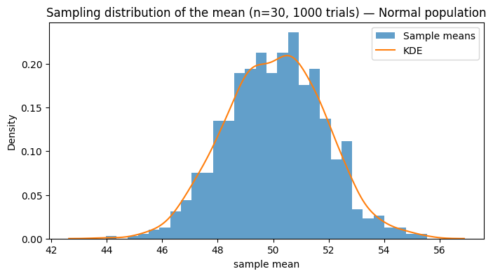
# Sampling distribution of the mean for Normal population
n = 30 # sample size
n_trials = 1000
sample_means = [np.mean(np.random.choice(pop_normal, size=n, replace=False)) for _ in range(n_trials)]
plt.figure(figsize=(8,4))
plt.hist(sample_means, bins=30, density=True, alpha=0.7, label='Sample means')
sns.kdeplot(sample_means, label='KDE')
plt.title(f'Sampling distribution of the mean (n={n}, {n_trials} trials) — Normal population')
plt.xlabel('sample mean')
plt.legend()
plt.show()
Normal: mean=50.020, std=10.012
Skewed: mean=40.019, std=10.002
Binary: mean=0.120, std=0.325
2 — Central Limit Theorem (CLT) visualization#
The CLT says that as sample size increases, the sampling distribution of the mean approaches a normal distribution, even if the population is not normal. Let’s demonstrate with our skewed population.
def show_clt(pop, sample_sizes=[5, 30, 100], trials=2000):
    fig, axes = plt.subplots(1, len(sample_sizes), figsize=(5*len(sample_sizes),4))
    for ax, n in zip(axes, sample_sizes):
        means = [np.mean(np.random.choice(pop, n, replace=False)) for _ in range(trials)]
        ax.hist(means, bins=30, density=True, alpha=0.6)
        sns.kdeplot(means, ax=ax)
        ax.set_title(f'n={n}, mean={np.mean(means):.2f}, sd={np.std(means, ddof=1):.2f}')
    plt.suptitle('CLT demonstration — sampling distribution of the mean (skewed population)')
    plt.tight_layout()
    plt.show()

show_clt(pop_skewed)
3 — One-sample z-test (known sigma)#
When the population standard deviation (sigma) is known and sample size is large, use the z-test.
Formula: $\(z = \frac{\bar{x} - \mu_0}{\sigma/\sqrt{n}}\)$
In practice, sigma is rarely known. This is mainly conceptual or used with very large samples.
def z_test_one_sample(x, mu0, sigma):
    n = len(x)
    xbar = np.mean(x)
    z = (xbar - mu0) / (sigma / sqrt(n))
    # two-tailed p-value
    p_two = 2 * (1 - stats.norm.cdf(abs(z)))
    return z, p_two

# Example: sample from normal population where true mu = 50
sample = np.random.choice(pop_normal, size=50, replace=False)
known_sigma = 10.0
z_stat, p_two = z_test_one_sample(sample, mu0=50, sigma=known_sigma)
print(f'Sample mean: {np.mean(sample):.3f}')
print(f'z-stat: {z_stat:.4f}, p-value (two-tailed): {p_two:.4f}')

# One-tailed p-value (H_a: mean > mu0)
p_one_greater = 1 - stats.norm.cdf(z_stat)
print(f'p-value (one-tailed, >): {p_one_greater:.4f}')
Sample mean: 51.156
z-stat: 0.8175, p-value (two-tailed): 0.4136
p-value (one-tailed, >): 0.2068
4 — One-sample t-test (unknown sigma)#
When sigma is unknown and sample size is small, use the t-distribution.
Formula: $\(t = \frac{\bar{x} - \mu_0}{s/\sqrt{n}}\)$
where s is the sample standard deviation. The t-distribution has “fatter tails” than the normal, giving us more conservative p-values for small samples.
def t_test_one_sample(x, mu0):
    n = len(x)
    xbar = np.mean(x)
    s = np.std(x, ddof=1)
    t_stat = (xbar - mu0) / (s / np.sqrt(n))
    p_two = 2 * (1 - t.cdf(abs(t_stat), df=n-1))
    return t_stat, p_two

# Small sample example
small_sample = np.random.choice(pop_normal, size=12, replace=False)
t_stat, p_two = t_test_one_sample(small_sample, mu0=50)
print(f'Sample size: {len(small_sample)}')
print(f'Sample mean: {np.mean(small_sample):.3f}, sample std: {np.std(small_sample, ddof=1):.3f}')
print(f't-stat (manual): {t_stat:.4f}, p-value: {p_two:.4f}')

# SciPy's ttest_1samp
scipy_t = stats.ttest_1samp(small_sample, popmean=50)
print(f'SciPy ttest_1samp: statistic={scipy_t.statistic:.4f}, pvalue={scipy_t.pvalue:.4f}')
Sample size: 12
Sample mean: 53.716, sample std: 7.945
t-stat (manual): 1.6202, p-value: 0.1335
SciPy ttest_1samp: statistic=1.6202, pvalue=0.1335
5 — Two-sample t-test (independent groups)#
Compare two independent groups. Two variants:
Student’s t-test: assumes equal variances (simpler)
Welch’s t-test: allows unequal variances (more robust, preferred)
# Two-sample example: compare two model accuracy samples
acc_A = np.random.normal(loc=0.78, scale=0.03, size=30)  # model A
acc_B = np.random.normal(loc=0.75, scale=0.03, size=30)  # model B

# Welch's t-test (default, unequal variance)
welch = stats.ttest_ind(acc_A, acc_B, equal_var=False)
print(f"Welch's t-test: t={welch.statistic:.4f}, p={welch.pvalue:.4f}")

# Student's t-test (equal variance)
student = stats.ttest_ind(acc_A, acc_B, equal_var=True)
print(f"Student's t-test: t={student.statistic:.4f}, p={student.pvalue:.4f}")

# Manual pooled t-statistic (for learning)
def pooled_ttest(x, y):
    nx, ny = len(x), len(y)
    sx2 = np.var(x, ddof=1)
    sy2 = np.var(y, ddof=1)
    sp2 = ((nx-1)*sx2 + (ny-1)*sy2) / (nx+ny-2)
    se = np.sqrt(sp2 * (1/nx + 1/ny))
    t_stat = (np.mean(x) - np.mean(y)) / se
    df = nx + ny - 2
    p_two = 2 * (1 - t.cdf(abs(t_stat), df))
    return t_stat, p_two, df

pt, pp, df = pooled_ttest(acc_A, acc_B)
print(f"Pooled t-test (manual): t={pt:.4f}, p={pp:.4f}, df={df}")
Welch's t-test: t=4.9767, p=0.0000
Student's t-test: t=4.9767, p=0.0000
Pooled t-test (manual): t=4.9767, p=0.0000, df=58
6 — Paired t-test#
Use paired t-test when observations are naturally paired (e.g., pre/post measurements, or same test set predicted by two classifiers). This accounts for within-subject correlation and often increases power.
# Paired example: pre/post
pre = np.random.normal(loc=1.0, scale=0.4, size=25)
post = pre + np.random.normal(loc=-0.15, scale=0.2, size=25)  # slight decrease

paired = stats.ttest_rel(pre, post)
print(f'Paired t-test: t={paired.statistic:.4f}, p={paired.pvalue:.4f}')

# Manual paired approach (differences)
diffs = pre - post
t_stat, p_two = t_test_one_sample(diffs, mu0=0)
print(f'Paired (manual via differences): t={t_stat:.4f}, p={p_two:.4f}')
Paired t-test: t=3.6152, p=0.0014
Paired (manual via differences): t=3.6152, p=0.0014
7 — One-tailed vs two-tailed tests#
Understanding the difference#
Two-tailed test:
Hypothesis: H1: μ ≠ μ0 (or p_A ≠ p_B, etc.)
Interpretation: Tests whether there is any difference (in either direction)
p-value: Probability of observing as extreme a result in either direction
Rejection region: Split between both tails (e.g., α/2 = 0.025 in each tail for α = 0.05)
When to use: When you have no prior expectation of direction, or when both directions matter
One-tailed test (e.g., right-tail):
Hypothesis: H1: μ > μ0 (or p_A < p_B for left-tail)
Interpretation: Tests whether the parameter is specifically greater (or less)
p-value: Probability of observing as extreme a result in the specified direction only
Rejection region: All α in one tail (e.g., α = 0.05 in right tail)
When to use: When you have a prior scientific/business expectation of direction (e.g., “new treatment should improve outcomes”)
Critical rule: Decide before looking at data!#
Choosing the tail after seeing the data inflates Type I error. This is called p-hacking or multiple comparisons and is scientifically invalid.
Mathematical relationship#
For a test statistic t: $\(p_{\text{two-tailed}} = 2 \times P(T > |t|)\)\( \)\(p_{\text{one-tailed}} = P(T > t) \text{ (for right-tail, } H_1: \mu > \mu_0\text{)}\)$
So one-tailed p-values are roughly half of two-tailed (when statistic is in the hypothesized direction).
Business/ML examples#
Two-tailed: Does model A differ from model B? (Don’t know which is better yet)
One-tailed right: Does feature X improve accuracy? (Directional: we expect improvement)
One-tailed left: Does the new manufacturing process reduce defects? (Directional: we expect reduction)
# Example: one-tailed from two-tailed
res = stats.ttest_ind(acc_A, acc_B, equal_var=False)
print(f'Two-tailed p: {res.pvalue:.4f}')

# Convert to one-tailed p (H_a: mean(A) > mean(B))
if res.statistic > 0:
    p_one_greater = res.pvalue / 2
else:
    p_one_greater = 1 - res.pvalue / 2

print(f'One-tailed p (A > B): {p_one_greater:.4f}')
Two-tailed p: 0.0000
One-tailed p (A > B): 0.0000
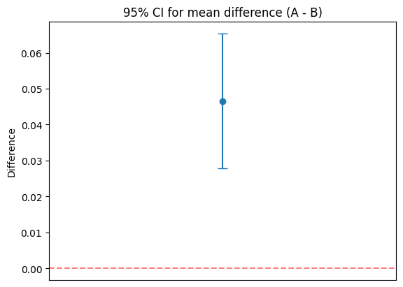
8 — Confidence intervals & relation to hypothesis tests#
If a 95% CI for a parameter does not include the null value (e.g., 0 for a difference), you would reject H0 at alpha=0.05.
# 95% CI for difference in two independent means (Welch)
mean_diff = np.mean(acc_A) - np.mean(acc_B)
se_diff = np.sqrt(np.var(acc_A, ddof=1)/len(acc_A) + np.var(acc_B, ddof=1)/len(acc_B))

# Use Welch-Satterthwaite df approximation
s1, s2 = np.var(acc_A, ddof=1), np.var(acc_B, ddof=1)
nx, ny = len(acc_A), len(acc_B)
df = (s1/nx + s2/ny)**2 / ((s1**2)/((nx**2)*(nx-1)) + (s2**2)/((ny**2)*(ny-1)))
ci_low = mean_diff - stats.t.ppf(0.975, df) * se_diff
ci_high = mean_diff + stats.t.ppf(0.975, df) * se_diff

print(f'Mean diff (A - B): {mean_diff:.4f}')
print(f'95% CI: ({ci_low:.4f}, {ci_high:.4f}), df~{df:.1f}')
print(f'CI includes 0: {ci_low <= 0 <= ci_high}')

# Plot
plt.errorbar([0], [mean_diff], yerr=[[mean_diff-ci_low],[ci_high-mean_diff]], fmt='o', capsize=5)
plt.axhline(0, color='red', linestyle='--', alpha=0.5)
plt.title('95% CI for mean difference (A - B)')
plt.xlim(-1,1)
plt.xticks([])
plt.ylabel('Difference')
plt.show()
Mean diff (A - B): 0.0466
95% CI: (0.0278, 0.0653), df~57.9
CI includes 0: False
9 — Effect size (Cohen’s d)#
Statistical significance ≠ practical significance. Always report effect sizes:
Rules of thumb: 0.2 (small), 0.5 (medium), 0.8 (large).
def cohen_d(x, y):
    nx, ny = len(x), len(y)
    sx2 = np.var(x, ddof=1)
    sy2 = np.var(y, ddof=1)
    sp = np.sqrt(((nx-1)*sx2 + (ny-1)*sy2) / (nx+ny-2))
    return (np.mean(x) - np.mean(y)) / sp

d = cohen_d(acc_A, acc_B)
interpretation = 'small' if abs(d)<0.5 else ('medium' if abs(d)<0.8 else 'large')
print(f"Cohen's d: {d:.4f} ({interpretation})")
Cohen's d: 1.2850 (large)
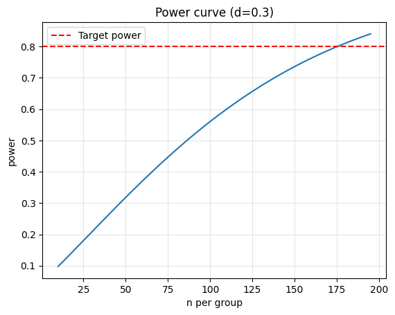
10 — Power analysis & sample size#
Determine sample size needed to detect an effect of size d with power 0.8 and alpha 0.05.
from statsmodels.stats.power import TTestIndPower

analysis = TTestIndPower()
eff_size = 0.3
alpha = 0.05
power = 0.8
n_required = analysis.solve_power(effect_size=eff_size, alpha=alpha, power=power, alternative='two-sided')
print(f'Required n per group: {np.ceil(n_required):.0f}')

# Power curve
sample_range = np.arange(10, 200, 5)
power_vals = [analysis.power(effect_size=eff_size, nobs1=n, alpha=alpha, ratio=1.0, alternative='two-sided') for n in sample_range]
plt.plot(sample_range, power_vals)
plt.axhline(0.8, color='red', linestyle='--', label='Target power')
plt.xlabel('n per group')
plt.ylabel('power')
plt.title(f'Power curve (d={eff_size})')
plt.legend()
plt.grid(alpha=0.3)
plt.show()
Required n per group: 176
11 — Parametric vs Non-Parametric Tests#
What are parametric tests?#
Parametric tests assume the data follows a specific distribution (usually normal/Gaussian). They estimate the parameters (mean, variance) of that distribution.
Examples:
t-tests (one-sample, two-sample, paired)
z-tests
ANOVA
Pearson correlation
Linear regression
Advantages:
✅ Higher power (more likely to detect true effects) when assumptions are satisfied
✅ Simpler formulas and faster computation
✅ Well-developed theory and software support
Disadvantages:
❌ Sensitive to violations of assumptions (non-normality, outliers, unequal variances)
❌ May give misleading p-values if assumptions fail
❌ Not suitable for small samples or ordinal/ranked data
What are non-parametric tests?#
Non-parametric tests make fewer assumptions about the underlying distribution. They typically work with ranks rather than raw values.
Examples:
Mann–Whitney U (instead of t-test for independent samples)
Wilcoxon signed-rank (instead of paired t-test)
Kruskal–Wallis (instead of one-way ANOVA)
Spearman correlation (instead of Pearson)
Advantages:
✅ Robust to outliers and distribution violations
✅ Work with ordinal data (ranks, ratings, scores)
✅ Valid for small samples
✅ Distribution-free (no assumption about the shape)
Disadvantages:
❌ Lower power than parametric tests when data is actually normal
❌ Less flexible; some advanced techniques unavailable
❌ Harder to interpret (working with ranks, not means)
Practical decision tree#
Check assumptions (normality, equal variances):
Use Shapiro–Wilk test (H0: data is normal)
Use Levene’s test (H0: equal variances)
If assumptions are met AND sample size is reasonable:
→ Use parametric test (higher power)
If assumptions violated OR small sample OR ordinal data:
→ Use non-parametric test (more robust)
When in doubt:
→ Report both and see if conclusions agree
→ Use permutation/bootstrap (modern, flexible)
Visual comparison: Normal vs Skewed data#
When data is normal, t-test and Mann–Whitney give similar results. When data is skewed or has outliers, Mann–Whitney is more reliable.
# Test assumptions before choosing parametric vs non-parametric

# Normality test (Shapiro-Wilk)
shapiro_a = stats.shapiro(acc_A)
shapiro_b = stats.shapiro(acc_B)
print('Normality tests (Shapiro-Wilk):')
print(f'  acc_A: W={shapiro_a.statistic:.4f}, p={shapiro_a.pvalue:.4f} => Normal: {shapiro_a.pvalue > 0.05}')
print(f'  acc_B: W={shapiro_b.statistic:.4f}, p={shapiro_b.pvalue:.4f} => Normal: {shapiro_b.pvalue > 0.05}')

# Equal variance test (Levene's)
levene = stats.levene(acc_A, acc_B)
print(f'\nLevene test (equal variances): F={levene.statistic:.4f}, p={levene.pvalue:.4f} => Equal vars: {levene.pvalue > 0.05}')

# Compare parametric vs non-parametric
print('\n--- Comparison of parametric vs non-parametric ---')

# Parametric: Welch's t-test
welch = stats.ttest_ind(acc_A, acc_B, equal_var=False)
print(f"Welch's t-test (parametric): t={welch.statistic:.4f}, p={welch.pvalue:.4f}")

# Non-parametric: Mann-Whitney U test
mw = stats.mannwhitneyu(acc_A, acc_B, alternative='two-sided')
print(f'Mann-Whitney U (non-parametric): U={mw.statistic:.4f}, p={mw.pvalue:.4f}')

print('\nNote: Both tests give similar conclusions when data is normal.')
print('If data were skewed, Mann-Whitney would be more reliable.')

# Wilcoxon signed-rank (paired)
print('\n--- Paired samples (pre/post) ---')
w = stats.wilcoxon(pre, post)
print(f'Wilcoxon signed-rank: statistic={w.statistic:.4f}, p={w.pvalue:.4f}')

# Compare with paired t-test
paired = stats.ttest_rel(pre, post)
print(f'Paired t-test: t={paired.statistic:.4f}, p={paired.pvalue:.4f}')
Normality tests (Shapiro-Wilk):
  acc_A: W=0.9456, p=0.1285 => Normal: True
  acc_B: W=0.9497, p=0.1658 => Normal: True

Levene test (equal variances): F=0.3003, p=0.5858 => Equal vars: True

--- Comparison of parametric vs non-parametric ---
Welch's t-test (parametric): t=4.9767, p=0.0000
Mann-Whitney U (non-parametric): U=740.0000, p=0.0000

Note: Both tests give similar conclusions when data is normal.
If data were skewed, Mann-Whitney would be more reliable.

--- Paired samples (pre/post) ---
Wilcoxon signed-rank: statistic=53.0000, p=0.0023
Paired t-test: t=3.6152, p=0.0014
12 — Permutation test & bootstrap#
Build the null distribution by shuffling labels (permutation) or resampling with replacement (bootstrap).
def permutation_test(x, y, n_permutations=5000, seed=RNG_SEED):
    rng = np.random.RandomState(seed)
    observed = np.mean(x) - np.mean(y)
    pooled = np.concatenate([x, y])
    stats_perm = []
    for _ in range(n_permutations):
        rng.shuffle(pooled)
        new_x = pooled[:len(x)]
        new_y = pooled[len(x):]
        stats_perm.append(np.mean(new_x) - np.mean(new_y))
    stats_perm = np.array(stats_perm)
    p_two = np.mean(np.abs(stats_perm) >= abs(observed))
    return observed, p_two, stats_perm

obs, pperm, null_dist = permutation_test(acc_A, acc_B)
print(f'Permutation test: observed diff={obs:.4f}, p={pperm:.4f}')

# Bootstrap CI
def bootstrap_ci(x, y, n_boot=2000, alpha=0.05, seed=RNG_SEED):
    rng = np.random.RandomState(seed)
    boot_diffs = []
    for _ in range(n_boot):
        bx = rng.choice(x, size=len(x), replace=True)
        by = rng.choice(y, size=len(y), replace=True)
        boot_diffs.append(np.mean(bx) - np.mean(by))
    ci_low = np.percentile(boot_diffs, 100*alpha/2)
    ci_high = np.percentile(boot_diffs, 100*(1-alpha/2))
    return np.mean(boot_diffs), ci_low, ci_high, boot_diffs

mean_boot, low_boot, high_boot, _ = bootstrap_ci(acc_A, acc_B)
print(f'Bootstrap CI: ({low_boot:.4f}, {high_boot:.4f})')
Permutation test: observed diff=0.0466, p=0.0000
Bootstrap CI: (0.0286, 0.0634)
13 — Multiple testing corrections#
When you run many tests, some will be significant by chance. Use corrections:
Bonferroni: controls family-wise error rate (FWER).
Benjamini–Hochberg: controls false discovery rate (FDR).
# Simulate multiple tests
rng = np.random.RandomState(RNG_SEED)
num_tests = 50
pvals = []
for i in range(num_tests):
    if i < 5:  # first 5 have real effect
        a = rng.normal(0.5, 0.2, size=30)
        b = rng.normal(0.0, 0.2, size=30)
    else:
        a = rng.normal(0.0, 0.2, size=30)
        b = rng.normal(0.0, 0.2, size=30)
    p = stats.ttest_ind(a, b, equal_var=False).pvalue
    pvals.append(p)

pvals = np.array(pvals)
_, p_bonf, _, _ = smm.multipletests(pvals, alpha=0.05, method='bonferroni')
_, p_bh, _, _ = smm.multipletests(pvals, alpha=0.05, method='fdr_bh')

print(f'Raw significant: {np.sum(pvals < 0.05)} / {num_tests}')
print(f'Bonferroni: {np.sum(p_bonf < 0.05)} / {num_tests}')
print(f'BH: {np.sum(p_bh < 0.05)} / {num_tests}')
Raw significant: 9 / 50
Bonferroni: 5 / 50
BH: 5 / 50
14 — ML applications: A/B tests & model comparison#
Practical examples: proportion z-test (conversion rates), McNemar (classifier disagreement).
# Proportion z-test (A/B conversions)
conv_A, n_A = 120, 1500
conv_B, n_B = 95, 1500

p_pool = (conv_A + conv_B) / (n_A + n_B)
z = (conv_A/n_A - conv_B/n_B) / np.sqrt(p_pool*(1-p_pool)*(1/n_A+1/n_B))
p_two = 2*(1 - stats.norm.cdf(abs(z)))

print(f'Proportion z-test: z={z:.4f}, p={p_two:.4f}')

# McNemar (classifier disagreement)
b, c = 30, 10  # b=A correct, B wrong; c=A wrong, B correct
chi2 = (abs(b - c) - 1)**2 / (b + c)
p_mcnemar = 1 - stats.chi2.cdf(chi2, df=1)

print(f'McNemar: chi2={chi2:.4f}, p={p_mcnemar:.4f}')
Proportion z-test: z=1.7696, p=0.0768
McNemar: chi2=9.0250, p=0.0027
15 — Addressing Multicollinearity: Variance Inflation Factor (VIF)#
What is multicollinearity?#
Multicollinearity occurs when two or more predictor variables in a regression model are highly correlated with each other. This causes problems:
Problems caused by multicollinearity:
❌ Large standard errors in regression coefficients → wider confidence intervals → weaker hypothesis tests
❌ Unstable estimates: small changes in data → big changes in coefficients
❌ Difficult interpretation: hard to isolate the effect of individual variables
❌ Poor predictions: model may overfit to training data despite good fit
❌ Misleading p-values: variables may appear non-significant when they actually are (due to inflated SE)
Example scenario:
Predicting house price from square footage and number of rooms
These two variables are highly correlated (larger house → more rooms)
The effect of each variable becomes unclear
What is Variance Inflation Factor (VIF)?#
VIF quantifies how much the variance of a regression coefficient is inflated due to multicollinearity.
where \(R_j^2\) is the R² from regressing variable \(j\) against all other predictors.
Interpretation:
VIF = 1: No correlation with other predictors (ideal)
1 < VIF < 5: Moderate correlation (usually acceptable)
VIF > 5: High multicollinearity (problematic) ← threshold often used
VIF > 10: Severe multicollinearity (must address)
Why is VIF useful?
Simple to compute and interpret
Each variable gets its own VIF score
Directly shows impact on standard errors: \(\text{SE}_{\text{with multicollinearity}} = \text{SE}_{\text{no multicollinearity}} \times \sqrt{\text{VIF}}\)
How to detect multicollinearity#
Correlation matrix: Look for correlations > 0.7 or < -0.7
Correlation heatmap: Visualize pairwise correlations
VIF test: Compute VIF for each predictor
How to address multicollinearity#
Option 1: Remove or combine variables
Drop one of the correlated variables
Combine correlated variables into a single index (e.g., PCA)
Option 2: Regularization
Use Ridge regression (L2 penalty) or Lasso (L1 penalty)
These shrink coefficients, reducing the effect of multicollinearity
Option 3: Collect more data
Larger sample size can reduce standard errors
Option 4: Reframe the problem
Use relative differences instead of absolute values
Center or standardize predictors
# Multicollinearity detection example

# Create a dataset with multicollinearity
np.random.seed(RNG_SEED)
n = 100
x1 = np.random.normal(0, 1, n)
x2 = 0.95 * x1 + 0.1 * np.random.normal(0, 1, n)  # highly correlated with x1
x3 = np.random.normal(0, 1, n)  # independent

y = 2*x1 + 3*x2 + 1*x3 + np.random.normal(0, 0.5, n)

# Create DataFrame
df_multi = pd.DataFrame({'x1': x1, 'x2': x2, 'x3': x3, 'y': y})

# Step 1: Correlation matrix
print('=== Correlation Matrix ===')
corr_matrix = df_multi.corr()
print(corr_matrix)

# Step 2: Visualize correlations (heatmap)
plt.figure(figsize=(6, 5))
sns.heatmap(corr_matrix, annot=True, cmap='coolwarm', center=0, square=True,
            vmin=-1, vmax=1, cbar_kws={'label': 'Correlation'})
plt.title('Correlation Heatmap (Multicollinearity Example)')
plt.tight_layout()
plt.show()

print(f'\n➤ Note: x1 and x2 are highly correlated (r = {corr_matrix.loc["x1", "x2"]:.3f})')

# Step 3: Compute VIF
from statsmodels.stats.outliers_influence import variance_inflation_factor

X = df_multi[['x1', 'x2', 'x3']]
vif_data = pd.DataFrame()
vif_data['Variable'] = X.columns
vif_data['VIF'] = [variance_inflation_factor(X.values, i) for i in range(X.shape[1])]

print('\n=== Variance Inflation Factor (VIF) ===')
print(vif_data)

# Interpretation
print('\nInterpretation:')
for idx, row in vif_data.iterrows():
    var = row['Variable']
    vif = row['VIF']
    if vif < 5:
        status = '✓ Acceptable'
    elif vif < 10:
        status = '⚠ Moderate multicollinearity'
    else:
        status = '✗ Severe multicollinearity'
    print(f"  {var}: VIF = {vif:.2f} — {status}")

# Step 4: Fit regression with multicollinearity
from sklearn.linear_model import LinearRegression

X_with_multi = df_multi[['x1', 'x2', 'x3']]
y_target = df_multi['y']

model_multi = LinearRegression()
model_multi.fit(X_with_multi, y_target)

print('\n=== Regression with Multicollinearity ===')
for i, coef in enumerate(model_multi.coef_):
    var_name = X_with_multi.columns[i]
    print(f"  {var_name}: coefficient = {coef:.4f}")

# Step 5: Compare with removing correlated variable
print('\n=== Regression without x2 (removing correlated variable) ===')
X_no_multi = df_multi[['x1', 'x3']]
model_no_multi = LinearRegression()
model_no_multi.fit(X_no_multi, y_target)

for i, coef in enumerate(model_no_multi.coef_):
    var_name = X_no_multi.columns[i]
    print(f"  {var_name}: coefficient = {coef:.4f}")

print('\n➤ Note: Removing the correlated variable x2 stabilizes the coefficient for x1')

# Step 6: Use regularization (Ridge regression)
from sklearn.linear_model import Ridge

print('\n=== Ridge Regression (L2 Regularization) ===')
ridge_model = Ridge(alpha=1.0)
ridge_model.fit(X_with_multi, y_target)

for i, coef in enumerate(ridge_model.coef_):
    var_name = X_with_multi.columns[i]
    print(f"  {var_name}: coefficient = {coef:.4f}")

print('\n➤ Note: Ridge regression handles multicollinearity by shrinking coefficients')
=== Correlation Matrix ===
          x1        x2        x3         y
x1  1.000000  0.995251 -0.151031  0.972934
x2  0.995251  1.000000 -0.160902  0.973579
x3 -0.151031 -0.160902  1.000000  0.047548
y   0.972934  0.973579  0.047548  1.000000
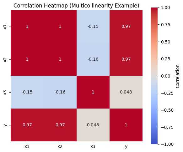
➤ Note: x1 and x2 are highly correlated (r = 0.995)

=== Variance Inflation Factor (VIF) ===
  Variable         VIF
0       x1  104.069386
1       x2  104.392490
2       x3    1.035209

Interpretation:
  x1: VIF = 104.07 — ✗ Severe multicollinearity
  x2: VIF = 104.39 — ✗ Severe multicollinearity
  x3: VIF = 1.04 — ✓ Acceptable

=== Regression with Multicollinearity ===
  x1: coefficient = 1.0710
  x2: coefficient = 3.9636
  x3: coefficient = 0.9650

=== Regression without x2 (removing correlated variable) ===
  x1: coefficient = 4.8736
  x3: coefficient = 0.9253

➤ Note: Removing the correlated variable x2 stabilizes the coefficient for x1

=== Ridge Regression (L2 Regularization) ===
  x1: coefficient = 2.0609
  x2: coefficient = 2.9089
  x3: coefficient = 0.9428

➤ Note: Ridge regression handles multicollinearity by shrinking coefficients
Takeaways#
Hypothesis Testing Core Concepts#
Hypothesis testing is a formal method to assess whether observed differences are “real” or due to random chance.
One-tailed vs two-tailed: choose directional vs non-directional before seeing data to avoid p-hacking.
Statistical ≠ practical significance: always report effect sizes and confidence intervals alongside p-values.
Test Selection#
Parametric tests (t-test, z-test): Higher power when normality holds; sensitive to violations
Non-parametric tests (Mann–Whitney, Wilcoxon): More robust to outliers/non-normality; suitable for ordinal data
Decision rule: Check assumptions (Shapiro-Wilk, Levene’s) → choose appropriately or use permutation/bootstrap
Model Validity & Diagnostics#
Multicollinearity inflates standard errors and destabilizes coefficients in regression models
VIF > 5: Indicates problematic multicollinearity; remedies include removing variables, regularization (Ridge/Lasso), or collecting more data
Assumptions matter: check normality, independence, equal variances; use non-parametric/permutation/bootstrap alternatives when assumptions fail
Best Practices in ML & Business#
Use hypothesis testing for A/B tests, model comparisons, feature validation, and quantifying uncertainty
Always report effect sizes (Cohen’s d), confidence intervals, and sample sizes alongside p-values
When running multiple tests, apply corrections (Bonferroni, Benjamini–Hochberg) to control error rates
Consider practical significance, not just statistical significance
Document and justify all decisions made before analyzing data
Further reading:
Introductory Statistics textbook (e.g., An Introduction to Statistical Learning)
A/B testing and experimental design tutorials
James et al., “An Introduction to Statistical Learning” — Chapter on Regression