🌲 Bagging, Random Forests & XGBoost#
Welcome to the forest of collective intelligence — where multiple models join forces to fix each other’s mistakes, kind of like an office where everyone double-checks the intern’s Excel formulas.
🎭 Why Ensemble Learning Exists#
One Decision Tree is fine — it’s interpretable and charming. But sometimes it gets a little… dramatic:
“Oh, you had one outlier? Let me completely change my entire structure!” 😱
To fix this, we combine multiple models to make predictions that are more stable, accurate, and less emotional.
👯♀️ Bagging: When Models Work in Parallel#
Bootstrap Aggregation (Bagging) is just a fancy way of saying:
“Let’s train a bunch of trees on slightly different samples and average their answers.”
Each tree gets a random subset of data and features, so they all have different perspectives. In the end, we average or vote their predictions.
🧃 Analogy:#
It’s like asking five friends to guess your age — one says 25, one says 27, one says “you look tired.” Average them, and boom: a much more accurate (and diplomatic) estimate.
⚙️ Python Example#
from sklearn.ensemble import BaggingClassifier
from sklearn.tree import DecisionTreeClassifier
bagging = BaggingClassifier(
base_estimator=DecisionTreeClassifier(),
n_estimators=10,
random_state=42
)
bagging.fit(X_train, y_train)
🌳 Random Forest: The Organized Forest Manager#
A Random Forest takes Bagging and adds a plot twist:
Each tree gets a random subset of features too. 🌈 This means not every tree focuses on the same things — avoiding groupthink.
Result? A model that’s more diverse, less correlated, and often more accurate.
🧠 Fun Fact:#
Random Forests are like a team of analysts — one obsessed with “age”, another with “income”, one just watching cat videos but still somehow contributing.
⚙️ Python Example#
from sklearn.ensemble import RandomForestClassifier
rf = RandomForestClassifier(
n_estimators=100,
max_depth=None,
random_state=42
)
rf.fit(X_train, y_train)
rf.score(X_test, y_test)
🎯 Use rf.feature_importances_ to find out which features actually matter
(spoiler: it’s never “favorite ice cream flavor”).
⚡ Boosting: The Model That Never Gives Up#
Now meet Boosting, the overachiever of the ML world.
Instead of training models independently, Boosting trains them sequentially:
Each model learns from the previous one’s mistakes.
Together, they become an unstoppable ensemble.
It’s like an employee who keeps getting feedback and actually improves — rare, but beautiful. 💪
🚀 XGBoost: The Caffeinated Genius#
Extreme Gradient Boosting (XGBoost) is the most famous booster — fast, powerful, and allergic to underfitting.
It uses:
Gradient boosting (to reduce errors efficiently)
Regularization (to prevent overfitting)
Parallelization (to train faster than your coffee brews)
⚙️ Python Example#
from xgboost import XGBClassifier
xgb = XGBClassifier(
n_estimators=200,
learning_rate=0.05,
max_depth=4,
random_state=42
)
xgb.fit(X_train, y_train)
⚠️ Warning: Once you use XGBoost, every other model feels like a flip phone 📞
🎨 Bagging vs Boosting (Cheat Sheet)#
Feature |
Bagging |
Boosting |
|---|---|---|
Training |
Parallel |
Sequential |
Goal |
Reduce variance |
Reduce bias |
Famous Models |
Random Forest |
AdaBoost, XGBoost, LightGBM |
Attitude |
“Let’s vote!” 🗳️ |
“Let’s improve!” 🔁 |
🧩 Business Example: Credit Risk Scoring#
Imagine you’re a bank deciding whether to approve a loan. Each model (tree) gives an opinion:
“High income → probably safe.”
“Low credit score → maybe risky.”
“Bought a luxury car last week → yikes.”
The Random Forest takes a vote. The XGBoost model learns over time which opinions were correct and adjusts. Result: lower default risk, higher profits, and fewer sleepless nights for your finance team.
🧠 Practice Exercise#
Try comparing the accuracy of:
A single Decision Tree
A Random Forest
An XGBoost model
Plot the feature importance for each and discuss:
Which features dominate?
Does boosting really help?
How does overfitting change with model complexity?
🌟 Coming Up Next#
Up next: we’ll peek behind the curtain of Feature Importance — where we learn which variables are secretly running the show. 🎭 Because in every business dataset, there’s always that one feature doing all the heavy lifting.
• Bootstrap Aggregating (Bagging)
• Random Forests and Feature Subsampling
• Boosting: AdaBoost, XGBoost (Extreme Gradient Boosting)
• Python: Implement AdaBoost with Weighted Errors
import numpy as np
import matplotlib.pyplot as plt
from matplotlib.colors import ListedColormap
from collections import Counter
import uuid
# Decision Tree Node
class Node:
def __init__(self, feature=None, threshold=None, left=None, right=None, value=None):
self.feature = feature
self.threshold = threshold
self.left = left
self.right = right
self.value = value
# Decision Tree Implementation
class DecisionTree:
def __init__(self, max_depth=3, min_samples_split=2):
self.max_depth = max_depth
self.min_samples_split = min_samples_split
self.root = None
def fit(self, X, y, feature_indices):
self.feature_indices = feature_indices
self.root = self._grow_tree(X, y, depth=0)
def _grow_tree(self, X, y, depth):
n_samples, n_features = X.shape
if (depth >= self.max_depth or n_samples < self.min_samples_split or len(np.unique(y)) == 1):
return Node(value=Counter(y).most_common(1)[0][0])
best_feature, best_threshold = self._best_split(X, y)
if best_feature is None:
return Node(value=Counter(y).most_common(1)[0][0])
left_idx = X[:, best_feature] <= best_threshold
right_idx = ~left_idx
left = self._grow_tree(X[left_idx], y[left_idx], depth + 1)
right = self._grow_tree(X[right_idx], y[right_idx], depth + 1)
return Node(best_feature, best_threshold, left, right)
def _best_split(self, X, y):
best_gain = -1
best_feature, best_threshold = None, None
n_samples, n_features = X.shape
for feature in self.feature_indices:
thresholds = np.unique(X[:, feature])
for threshold in thresholds:
left_idx = X[:, feature] <= threshold
right_idx = ~left_idx
if sum(left_idx) == 0 or sum(right_idx) == 0:
continue
gain = self._information_gain(y, left_idx, right_idx)
if gain > best_gain:
best_gain = gain
best_feature = feature
best_threshold = threshold
return best_feature, best_threshold
def _information_gain(self, y, left_idx, right_idx):
parent_entropy = self._entropy(y)
n = len(y)
n_l, n_r = sum(left_idx), sum(right_idx)
if n_l == 0 or n_r == 0:
return 0
child_entropy = (n_l / n) * self._entropy(y[left_idx]) + (n_r / n) * self._entropy(y[right_idx])
return parent_entropy - child_entropy
def _entropy(self, y):
hist = np.bincount(y)
ps = hist / len(y)
return -np.sum([p * np.log2(p) for p in ps if p > 0])
def predict(self, X):
return np.array([self._traverse_tree(x, self.root) for x in X])
def _traverse_tree(self, x, node):
if node.value is not None:
return node.value
if x[node.feature] <= node.threshold:
return self._traverse_tree(x, node.left)
return self._traverse_tree(x, node.right)
# Random Forest Implementation
class RandomForest:
def __init__(self, n_trees=3, max_depth=3, min_samples_split=2, n_features=None):
self.n_trees = n_trees
self.max_depth = max_depth
self.min_samples_split = min_samples_split
self.n_features = n_features
self.trees = []
def fit(self, X, y):
self.trees = []
n_samples, n_features = X.shape
if self.n_features is None:
self.n_features = int(np.sqrt(n_features))
for _ in range(self.n_trees):
# Bootstrap sampling
idx = np.random.choice(n_samples, n_samples, replace=True)
X_sample, y_sample = X[idx], y[idx]
feature_indices = np.random.choice(n_features, self.n_features, replace=False)
tree = DecisionTree(self.max_depth, self.min_samples_split)
tree.fit(X_sample, y_sample, feature_indices)
self.trees.append((tree, feature_indices))
def predict(self, X):
predictions = np.array([tree.predict(X) for tree, _ in self.trees])
return np.apply_along_axis(lambda x: Counter(x).most_common(1)[0][0], axis=0, arr=predictions)
# Function to plot decision boundary
def plot_decision_boundary(X, y, model, title, test_points=None):
x_min, x_max = X[:, 0].min() - 1, X[:, 0].max() + 1
y_min, y_max = X[:, 1].min() - 1, X[:, 1].max() + 1
xx, yy = np.meshgrid(np.arange(x_min, x_max, 0.1), np.arange(y_min, y_max, 0.1))
Z = model.predict(np.c_[xx.ravel(), yy.ravel()])
Z = Z.reshape(xx.shape)
plt.contourf(xx, yy, Z, alpha=0.3, cmap=ListedColormap(['#FFAAAA', '#AAAAFF']))
plt.scatter(X[:, 0], X[:, 1], c=y, edgecolor='k', cmap=ListedColormap(['#FF0000', '#0000FF']))
if test_points is not None:
plt.scatter(test_points[:, 0], test_points[:, 1], c='green', s=100, marker='*', label='Test Points')
plt.title(title)
plt.xlabel('Feature 1')
plt.ylabel('Feature 2')
plt.legend()
# Function to plot tree structure
def plot_tree(node, depth=0, pos=(0, 0), ax=None, feature_names=None):
if ax is None:
fig, ax = plt.subplots(figsize=(8, 6))
if node.value is not None:
ax.text(pos[0], pos[1], f"Class {node.value}", bbox=dict(facecolor='lightgreen', edgecolor='black'))
return
ax.text(pos[0], pos[1], f"X[{feature_names[node.feature]}] <= {node.threshold:.2f}",
bbox=dict(facecolor='lightblue', edgecolor='black'))
if node.left:
ax.plot([pos[0], pos[0] - 0.3/(depth+1)], [pos[1] - 0.1, pos[1] - 0.3], 'k-')
plot_tree(node.left, depth + 1, (pos[0] - 0.3/(depth+1), pos[1] - 0.3), ax, feature_names)
if node.right:
ax.plot([pos[0], pos[0] + 0.3/(depth+1)], [pos[1] - 0.1, pos[1] - 0.3], 'k-')
plot_tree(node.right, depth + 1, (pos[0] + 0.3/(depth+1), pos[1] - 0.3), ax, feature_names)
# Main execution
if __name__ == "__main__":
# Generate synthetic data
np.random.seed(42)
X = np.vstack([
np.random.normal([2, 2], 0.5, (50, 2)),
np.random.normal([4, 4], 0.5, (50, 2))
])
y = np.array([0] * 50 + [1] * 50)
test_points = np.array([[2.5, 2.5], [3.5, 3.5], [4.5, 4.5]])
# Train Random Forest
rf = RandomForest(n_trees=3, max_depth=2, n_features=2)
rf.fit(X, y)
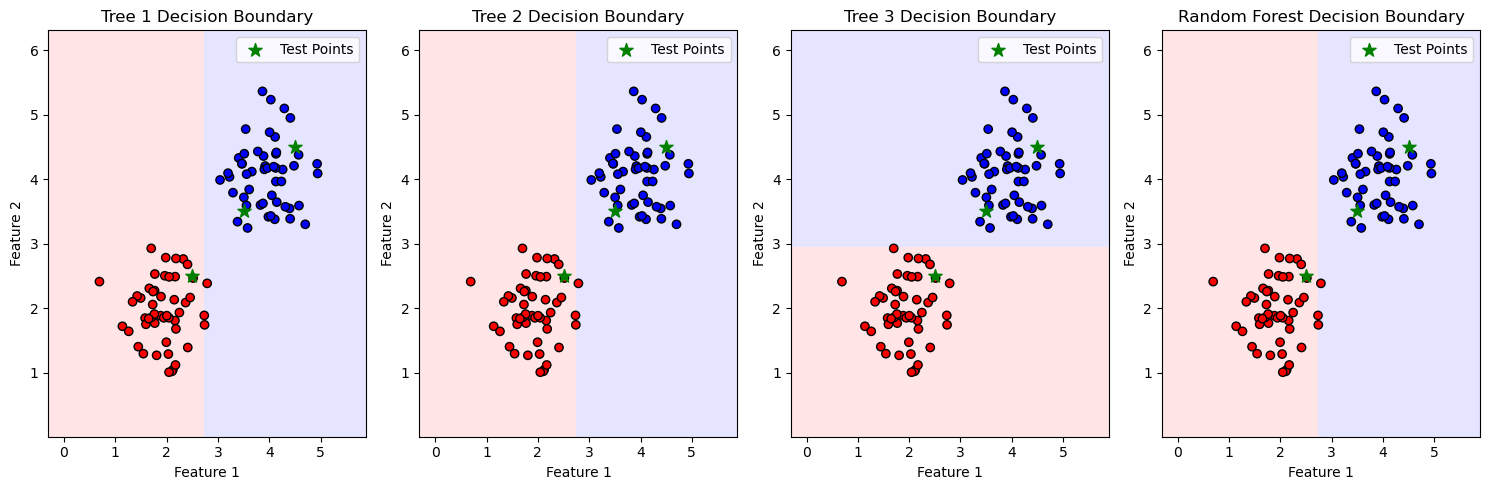
# Plot decision boundaries for each tree and the ensemble
plt.figure(figsize=(15, 5))
for i, (tree, feature_indices) in enumerate(rf.trees):
plt.subplot(1, 4, i + 1)
plot_decision_boundary(X, y, tree, f"Tree {i+1} Decision Boundary", test_points)
plt.subplot(1, 4, 4)
plot_decision_boundary(X, y, rf, "Random Forest Decision Boundary", test_points)
plt.tight_layout()
plt.savefig('decision_boundaries.png')
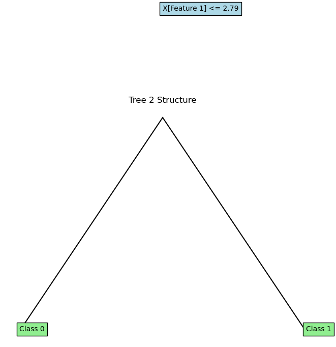
# Plot tree structures
for i, (tree, feature_indices) in enumerate(rf.trees):
plt.figure(figsize=(8, 6))
plot_tree(tree.root, feature_names=['Feature 1', 'Feature 2'])
plt.title(f"Tree {i+1} Structure")
plt.axis('off')
plt.savefig(f'tree_structure_{i+1}.png')
# Predict and print results for test points
predictions = rf.predict(test_points)
print("Test Point Predictions:")
for i, point in enumerate(test_points):
print(f"Point {point}: Predicted Class {predictions[i]}")
Test Point Predictions:
Point [2.5 2.5]: Predicted Class 0
Point [3.5 3.5]: Predicted Class 1
Point [4.5 4.5]: Predicted Class 1
<Figure size 800x600 with 0 Axes>

<Figure size 800x600 with 0 Axes>
<Figure size 800x600 with 0 Axes>

pip install xgboost
import numpy as np
import matplotlib.pyplot as plt
from matplotlib.animation import FuncAnimation
from sklearn.datasets import make_moons
from sklearn.model_selection import train_test_split
from sklearn.ensemble import RandomForestClassifier
from sklearn.tree import DecisionTreeClassifier
from xgboost import XGBClassifier
from IPython.display import HTML
# Generate synthetic 2D classification dataset
X, y = make_moons(n_samples=200, noise=0.3, random_state=42)
X_train, X_test, y_train, y_test = train_test_split(X, y, test_size=0.3, random_state=42)
n_samples = len(y_train)
# Create meshgrid for decision boundary visualization
x_min, x_max = X[:, 0].min() - 1, X[:, 0].max() + 1
y_min, y_max = X[:, 1].min() - 1, X[:, 1].max() + 1
xx, yy = np.meshgrid(np.arange(x_min, x_max, 0.01), np.arange(y_min, y_max, 0.01))
X_grid = np.c_[xx.ravel(), yy.ravel()]
# Random Forest setup
rf = RandomForestClassifier(n_estimators=100, random_state=42)
rf.fit(X_train, y_train)
rf_probabilities = []
for k in range(1, 101):
trees = rf.estimators_[:k]
probs = np.mean([tree.predict_proba(X_grid)[:, 1] for tree in trees], axis=0)
rf_probabilities.append(probs)
# XGBoost setup
xgb = XGBClassifier(n_estimators=100, random_state=42, eval_metric='logloss')
xgb.fit(X_train, y_train)
xgb_probabilities = []
for k in range(1, 101):
xgb_temp = XGBClassifier(n_estimators=k, random_state=42, eval_metric='logloss')
xgb_temp.fit(X_train, y_train)
probs = xgb_temp.predict_proba(X_grid)[:, 1]
xgb_probabilities.append(probs)
# AdaBoost with Weighted Errors implementation
def adaboost(X, y, n_estimators):
y_ab = 2 * y - 1 # Convert labels to -1 and 1
w = np.ones(len(y)) / len(y)
models, alphas, weights_list = [], [], [w.copy()]
for _ in range(n_estimators):
clf = DecisionTreeClassifier(max_depth=1)
clf.fit(X, y_ab, sample_weight=w)
pred = clf.predict(X)
err = np.sum(w * (pred != y_ab)) / np.sum(w)
alpha = 0.5 * np.log((1 - err) / err)
w = w * np.exp(-alpha * y_ab * pred)
w /= np.sum(w)
models.append(clf)
alphas.append(alpha)
weights_list.append(w.copy())
return models, alphas, weights_list
adaboost_models, adaboost_alphas, weights_list = adaboost(X_train, y_train, 100)
h_m = [model.predict(X_grid) for model in adaboost_models]
adaboost_probabilities = []
S = np.zeros(len(X_grid))
for alpha, h in zip(adaboost_alphas, h_m):
S += alpha * h
prob = 1 / (1 + np.exp(-S))
adaboost_probabilities.append(prob)
# Set up the figure and subplots
fig, axes = plt.subplots(1, 3, figsize=(15, 5))
axes[0].set_title('Random Forest')
axes[1].set_title('XGBoost')
axes[2].set_title('AdaBoost with Weighted Errors')
# Initial plots
pcm_rf = axes[0].pcolormesh(xx, yy, rf_probabilities[0].reshape(xx.shape), cmap='RdBu', shading='auto')
pcm_xgb = axes[1].pcolormesh(xx, yy, xgb_probabilities[0].reshape(xx.shape), cmap='RdBu', shading='auto')
pcm_ab = axes[2].pcolormesh(xx, yy, adaboost_probabilities[0].reshape(xx.shape), cmap='RdBu', shading='auto')
scatter_rf = axes[0].scatter(X_train[:, 0], X_train[:, 1], c=y_train, cmap='RdBu', s=20, edgecolor='k')
scatter_xgb = axes[1].scatter(X_train[:, 0], X_train[:, 1], c=y_train, cmap='RdBu', s=20, edgecolor='k')
s_ab = 50 * weights_list[0] * n_samples
scatter_ab = axes[2].scatter(X_train[:, 0], X_train[:, 1], c=y_train, cmap='RdBu', s=s_ab, edgecolor='k')
# Update function for animation
def update(k):
pcm_rf.set_array(rf_probabilities[k].ravel())
pcm_xgb.set_array(xgb_probabilities[k].ravel())
pcm_ab.set_array(adaboost_probabilities[k].ravel())
s_ab = 50 * weights_list[k + 1] * n_samples
scatter_ab.set_sizes(s_ab)
fig.suptitle(f'Number of Estimators: {k + 1}')
return pcm_rf, pcm_xgb, pcm_ab, scatter_ab
# Create and display animation
anim = FuncAnimation(fig, update, frames=100, interval=200, blit=False)
plt.close() # Prevent static display of the initial frame
HTML(anim.to_jshtml())