Gradient Descent Variants#
Teaching your model to climb down the mountain of loss without tripping over itself. 😆
🎯 The Big Idea#
Every model has one goal in life:
“Find the set of parameters that minimize the loss function.”
Gradient Descent (GD) is the personal trainer that helps it get there — step by step, calorie by calorie (and sometimes rage quit by rage quit 💢).
[ \theta_{new} = \theta_{old} - \eta \cdot \nabla L(\theta) ]
Where:
( \theta ) = parameters of the model
( \eta ) = learning rate (how fast we step)
( \nabla L(\theta) ) = gradient (direction of steepest descent)
🏔️ Visual Intuition#
Imagine you’re blindfolded, standing on a mountain in thick fog 🌫️. You can only feel the slope beneath your feet.
So, at each step you:
Check which way is downhill (gradient).
Take a small step that way (learning rate).
Repeat until you find the valley (minimum).
“That’s literally what gradient descent is — a blindfolded optimization hiker with a calculator.” 🤓
⚙️ Types of Gradient Descent#
There are three main variants — each with a distinct personality:
Variant |
Description |
Personality Type |
|---|---|---|
Batch GD |
Uses the entire dataset for each update |
The calm, methodical accountant 🧾 |
Stochastic GD (SGD) |
Uses one sample per update |
The over-caffeinated intern ☕ |
Mini-Batch GD |
Uses a subset (batch) of samples |
The zen project manager 🧘 |
Let’s meet each one 👇
🧮 1️⃣ Batch Gradient Descent#
Process:
Compute gradient using all training data before each step.
Very accurate but painfully slow.
💬 Imagine waiting for the entire company to reply to an email before taking the next step. 😅
✅ Pros: Stable convergence ❌ Cons: Time-consuming, memory-heavy
⚡ 2️⃣ Stochastic Gradient Descent (SGD)#
Process:
Update the weights after every sample.
Fast but noisy — the loss curve looks like your Wi-Fi signal. 📶
💬 SGD’s life motto:
“Why walk carefully when you can sprint downhill screaming?” 🏃💨
✅ Pros: Quick updates, faster convergence initially ❌ Cons: High variance, unpredictable path
☯️ 3️⃣ Mini-Batch Gradient Descent#
Process:
Split data into batches (e.g. 32 or 64 samples).
Update weights after each mini-batch.
💬 Think of it as yoga for your optimizer — flexible, balanced, and consistent. 🧘♂️
✅ Pros: Efficient, stable ❌ Cons: Requires tuning batch size (too big = slow, too small = noisy)
🎢 Comparing the Chaos#
Type |
Update Frequency |
Stability |
Speed |
Noise Level |
|---|---|---|---|---|
Batch |
Once per epoch |
Very High |
Low |
🚫 None |
SGD |
Every sample |
Low |
High |
🔥 Extreme |
Mini-Batch |
Every few samples |
Moderate |
Moderate |
⚖️ Balanced |
“In business terms: Batch GD = corporate bureaucracy, SGD = chaotic startup, Mini-Batch = well-run scale-up.” 🚀
🧠 Example Visualization#
Here’s how they behave differently on the same loss surface:
🎨 Interpretation:
Batch GD: smooth and calm 🧘♀️
SGD: chaotic and jittery ⚡
Mini-Batch: a chill balance of both 😎
🧩 Practice Corner#
Challenge |
Hint |
|---|---|
1️⃣ Simulate your own GD updates on a quadratic loss |
Try |
2️⃣ Add random noise to simulate SGD’s “mood swings” |
Use |
3️⃣ Plot the path of each variant on the same loss curve |
Compare visually |
4️⃣ Try different batch sizes (8, 32, 128) |
Watch the trade-off |
💬 Final Thought#
“Gradient Descent is proof that slow progress in the right direction still gets you to the valley.” 🌄
Whether you’re a model, a manager, or a confused human — just keep descending.
🔜 Next Up#
➡️ Advanced Optimizers (Adam, etc.) We’ll meet the supercharged versions of GD — the ones that remember the past, adapt the future, and occasionally overshoot into glory. 💥
Why Gradient Descent?#
Scalability: Gradient descent processes data iteratively (e.g., in mini-batches), requiring memory only for a small subset of data at a time (e.g., \(128 \times 500 \times 8\) bytes = \(0.061\) MB per batch).
Speed: For large datasets, computing the inverse of \(X^TX\) is computationally expensive (\(O(n^3)\)), while gradient descent is linear in the number of iterations.
Real-time updates: In finance, new data (e.g., trades) arrives constantly. Gradient descent can update the model incrementally, while the normal equation requires recomputing everything.
Thus, gradient descent is preferred for large-scale financial modeling, risk management, or customer segmentation in business applications where datasets are massive and computational resources are limited.
Introduction to Gradient Descent#
Gradient descent is an iterative optimization algorithm used to minimize a function, typically a loss/cost function in machine learning. It adjusts parameters by moving in the direction of the steepest descent, as defined by the negative gradient of the function.
1. Differentiation in Gradient Descent#
To minimize a function \(J(\theta)\), where \(\theta\) represents model parameters, gradient descent uses derivatives to determine the slope of the cost function at a given point. The derivative \(\frac{\partial J(\theta)}{\partial \theta_j}\) quantifies how \(J(\theta)\) changes as \(\theta_j\) changes.
The update rule for gradient descent is: $\( \theta_j := \theta_j - \alpha \frac{\partial J(\theta)}{\partial \theta_j} \)$ where:
\(\alpha\) is the learning rate (step size).
\(\frac{\partial J(\theta)}{\partial \theta_j}\) is the partial derivative of \(J(\theta)\) with respect to \(\theta_j\).
2. Squared Error Cost Function#
A common loss function is the mean squared error (MSE), used in linear regression. For \(m\) training examples, it measures the average squared difference between predicted values \(h_\theta(x^{(i)})\) and actual values \(y^{(i)}\): $\( J(\theta) = \frac{1}{2m} \sum_{i=1}^m \left( h_\theta(x^{(i)}) - y^{(i)} \right)^2 \)$ Here:
\(h_\theta(x^{(i)}) = \theta^T x^{(i)}\) (linear model prediction).
The \(\frac{1}{2}\) term simplifies derivatives.
3. Combining Gradient Descent and Squared Error#
To minimize \(J(\theta)\), we compute the gradient of the squared error term.
Derivative of the Squared Error#
For a single parameter \(\theta_j\), the partial derivative of \(J(\theta)\) is: $\( \frac{\partial J(\theta)}{\partial \theta_j} = \frac{1}{m} \sum_{i=1}^m \left( h_\theta(x^{(i)}) - y^{(i)} \right) x_j^{(i)} \)\( This derivative is used in the gradient descent update rule: \)\( \theta_j := \theta_j - \alpha \cdot \frac{1}{m} \sum_{i=1}^m \left( h_\theta(x^{(i)}) - y^{(i)} \right) x_j^{(i)} \)$
Intuition#
Squared error: Penalizes large errors quadratically, ensuring smooth optimization.
Gradient: Points in the direction of steepest ascent, so moving in the negative gradient direction minimizes the error.
Summary#
Gradient descent iteratively adjusts parameters \(\theta\) using the gradient of the squared error. The squared error’s convexity guarantees convergence to a global minimum (for linear models), and differentiation provides the necessary direction for updates.
import numpy as np
import matplotlib.pyplot as plt
# Desired velocity
v_star = 10
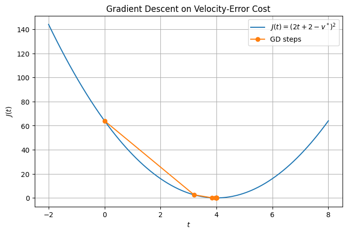
# Define cost and its gradient
def J(t):
return (2*t + 2 - v_star)**2
def dJ(t):
return 4 * (2*t + 2 - v_star)
# Plot J(t)
t_vals = np.linspace(-2, 8, 400)
J_vals = J(t_vals)
plt.figure(figsize=(8, 5))
plt.plot(t_vals, J_vals, label='$J(t)=(2t+2-v^*)^2$')
# Gradient descent path
t = 0.0
eta = 0.1
path = [t]
for _ in range(10):
t = t - eta * dJ(t)
path.append(t)
plt.plot(path, J(np.array(path)), 'o-', label='GD steps')
plt.title("Gradient Descent on Velocity‐Error Cost")
plt.xlabel('$t$')
plt.ylabel('$J(t)$')
plt.legend()
plt.grid(True)
plt.show()
import numpy as np
import matplotlib.pyplot as plt
# Define the cost function and its derivative
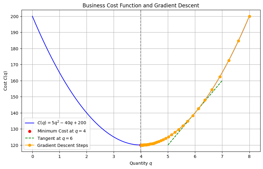
def C(q):
return 5*q**2 - 40*q + 200
def dC(q):
return 10*q - 40
# Define quantity values
q_vals = np.linspace(0, 8, 400)
cost_vals = C(q_vals)
# Plot the cost function
plt.figure(figsize=(10, 6))
plt.plot(q_vals, cost_vals, label='$C(q) = 5q^2 - 40q + 200$', color='blue')
# Mark the minimum point
q_min = 4
plt.scatter([q_min], [C(q_min)], color='red', label='Minimum Cost at $q=4$')
plt.axvline(x=q_min, linestyle='--', color='gray')
# Tangent line at q = 6
q_tangent = 6
slope = dC(q_tangent)
y_tangent = C(q_tangent)
q_range = np.linspace(q_tangent - 1, q_tangent + 1, 100)
tangent_line = slope * (q_range - q_tangent) + y_tangent
plt.plot(q_range, tangent_line, linestyle='--', color='green', label='Tangent at $q=6$')
# Gradient descent visualization
q = 8
eta = 0.01
q_path = [q]
for _ in range(50):
q = q - eta * dC(q)
q_path.append(q)
plt.plot(q_path, C(np.array(q_path)), 'o-', label='Gradient Descent Steps', color='orange')
# Final plot settings
plt.title("Business Cost Function and Gradient Descent")
plt.xlabel("Quantity $q$")
plt.ylabel("Cost $C(q)$")
plt.grid(True)
plt.legend()
plt.show()
import numpy as np
import matplotlib.pyplot as plt
from matplotlib.animation import FuncAnimation, PillowWriter
# Cost function and derivative
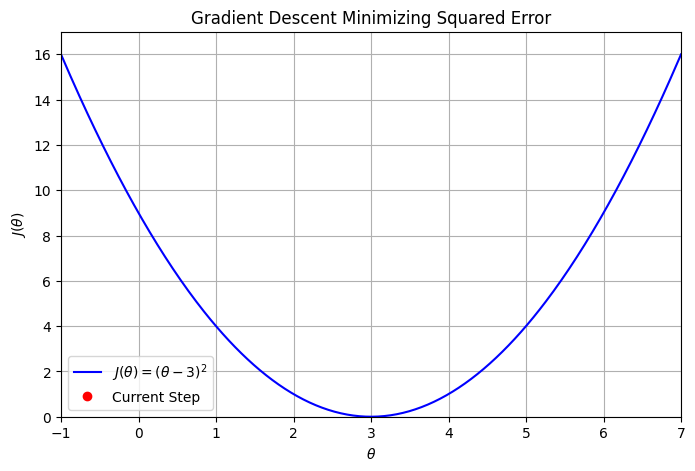
def J(theta):
return (theta - 3) ** 2
def dJ(theta):
return 2 * (theta - 3)
# Hyperparameters
alpha = 0.1
theta = 0.0
steps = 50
# Record history for animation
thetas = [theta]
costs = [J(theta)]
# Perform gradient descent
for _ in range(steps):
theta = theta - alpha * dJ(theta)
thetas.append(theta)
costs.append(J(theta))
# Setup figure and axis
theta_vals = np.linspace(-1, 7, 400)
cost_vals = J(theta_vals)
fig, ax = plt.subplots(figsize=(8, 5))
ax.plot(theta_vals, cost_vals, 'b-', label=r'$J(\theta) = (\theta - 3)^2$')
point, = ax.plot([], [], 'ro', label='Current Step')
text = ax.text(0.05, 0.9, '', transform=ax.transAxes)
ax.set_xlim(-1, 7)
ax.set_ylim(0, max(cost_vals) + 1)
ax.set_xlabel(r'$\theta$')
ax.set_ylabel(r'$J(\theta)$')
ax.set_title('Gradient Descent Minimizing Squared Error')
ax.grid(True)
ax.legend()
# Initialization function
def init():
point.set_data([], [])
text.set_text('')
return point, text
# Update function
def update(frame):
x = [thetas[frame]]
y = [costs[frame]]
point.set_data(x, y)
text.set_text(f'Step: {frame}\nθ: {x[0]:.4f}\nJ(θ): {y[0]:.4f}')
return point, text
# Create animation
ani = FuncAnimation(fig, update, frames=len(thetas), init_func=init, blit=False, interval=300)
# 10. Save as GIF
ani.save('gradientdescent.gif', writer=PillowWriter(fps=10))
# 11. Display saved GIF inside notebook
from IPython.display import Image
Image(filename="gradientdescent.gif")
Gradient descent#
Requires the calculation of \(m\) gradients in each step.
import numpy as np
import matplotlib.pyplot as plt
from matplotlib.animation import FuncAnimation, PillowWriter
# Cost function and derivative
def J(theta):
return (theta - 3)**2
def dJ(theta):
return 2 * (theta - 3)
# Hyperparameters
alpha = 0.1
theta = 0.0
steps = 50
thetas = [theta]
costs = [J(theta)]
# Gradient descent
for _ in range(steps):
theta = theta - alpha * dJ(theta)
thetas.append(theta)
costs.append(J(theta))
# Plot setup
theta_vals = np.linspace(-1, 7, 400)
cost_vals = J(theta_vals)
fig, ax = plt.subplots(figsize=(8, 5))
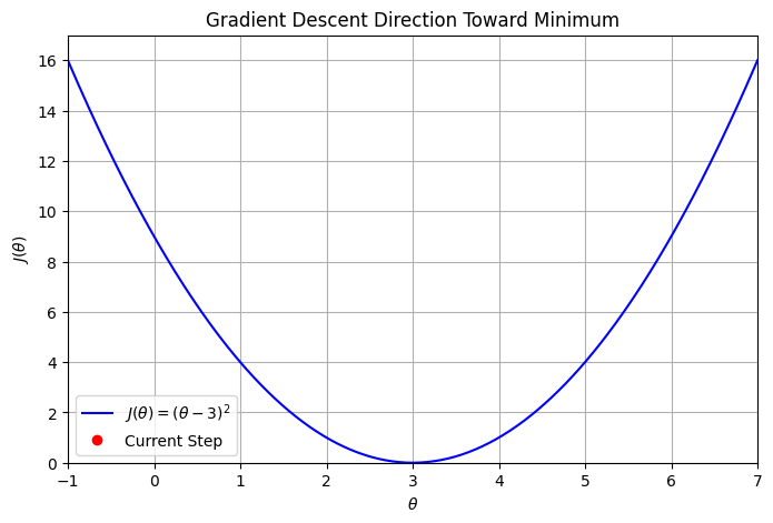
ax.plot(theta_vals, cost_vals, 'b-', label=r'$J(\theta) = (\theta - 3)^2$')
point, = ax.plot([], [], 'ro', label='Current Step')
arrow = ax.annotate('', xy=(0, 0), xytext=(0, 0),
arrowprops=dict(arrowstyle='->', color='red', lw=2))
text = ax.text(0.05, 0.9, '', transform=ax.transAxes)
ax.set_xlim(-1, 7)
ax.set_ylim(0, max(cost_vals) + 1)
ax.set_xlabel(r'$\theta$')
ax.set_ylabel(r'$J(\theta)$')
ax.set_title('Gradient Descent Direction Toward Minimum')
ax.grid(True)
ax.legend()
# Init function
def init():
point.set_data([], [])
arrow.set_position((0, 0))
arrow.xy = (0, 0)
text.set_text('')
return point, arrow, text
# Update function
def update(frame):
x = thetas[frame]
y = costs[frame]
point.set_data([x], [y])
# Draw arrow if not last frame
if frame < len(thetas) - 1:
next_x = thetas[frame + 1]
next_y = costs[frame + 1]
arrow.xy = (next_x, next_y)
arrow.set_position((x, y))
else:
arrow.xy = (x, y)
arrow.set_position((x, y))
text.set_text(f"Step: {frame}\nθ: {x:.4f}\nJ(θ): {y:.4f}")
return point, arrow, text
# Animate
ani = FuncAnimation(fig, update, frames=len(thetas), init_func=init, blit=False, interval=300)
# 10. Save as GIF
ani.save('gradientdescentarrow.gif', writer=PillowWriter(fps=10))
# 11. Display saved GIF inside notebook
from IPython.display import Image
Image(filename="gradientdescentarrow.gif")
# Your code here