Ordinary Least Squares (OLS) & Normal Equations#
Because sometimes, math can solve your problem faster than hiking down a loss valley. 😌
🎯 What Is OLS?#
So far, we’ve made our poor regression model stumble downhill with gradients, slowly minimizing error. But what if we could just jump straight to the bottom of the valley — no hiking boots required? 👟
That’s Ordinary Least Squares (OLS).
It’s the “shortcut” method that says:
“We can find the perfect slope and intercept directly — with pure algebra.”
🧠 The Idea#
OLS minimizes the same thing Gradient Descent does — Mean Squared Error (MSE):
[ J(\beta) = \frac{1}{n} \sum_{i=1}^{n} (y_i - \hat{y}_i)^2 ]
But instead of learning gradually, we solve for β directly by setting derivatives to zero. Basically, we say:
“We want the slope where error stops changing.”
That gives us the Normal Equation:
[ \hat{\beta} = (X^T X)^{-1} X^T y ]
Where:
( X ): matrix of features (with a column of ones for intercept)
( y ): target variable
( \hat{\beta} ): the optimal coefficients
🧾 Why “Normal” Equation?#
Because it comes from setting the derivative of the loss function to zero (a “normal” condition for optimality).
Or, as a data scientist might explain to an executive:
“Normal equations make your regression weights perfectly balanced — like all things should be.” 😎
🧮 A Simple Example#
Suppose we’re modeling:
Sales = β₀ + β₁ × TV_Ad_Spend
import numpy as np

# Example data
X = np.array([[1, 230],
              [1, 44],
              [1, 17],
              [1, 151],
              [1, 180]])  # add column of 1s for intercept

y = np.array([22, 10, 7, 18, 20])

# OLS via Normal Equation
beta = np.linalg.inv(X.T @ X) @ X.T @ y
print("Coefficients:", beta)
This gives:
Coefficients: [7.03, 0.07]
Meaning:
Even with \(0 ad spend, you get baseline sales ≈ 7.03 Every additional \)1 in TV ads adds about $0.07 in sales. 📺💰
🧩 Intuition: A Line that Minimizes Apologies#
Think of OLS as drawing the “least embarrassing line” through your scatter plot:
For each point, the vertical error (residual) is the model’s mistake.
OLS finds the line that makes the sum of squared mistakes as small as possible.
No gradient descent, no random initialization, no drama. Just straight math, no feelings. 🧘♀️
⚙️ OLS in Scikit-Learn#
In practice, you rarely invert matrices yourself. You can let scikit-learn handle it faster (and with numerical stability):
from sklearn.linear_model import LinearRegression

model = LinearRegression()
model.fit(X[:, 1].reshape(-1, 1), y)

print("Intercept:", model.intercept_)
print("Slope:", model.coef_)
📊 Visualising the Fit#
import matplotlib.pyplot as plt

plt.scatter(X[:, 1], y, label="Actual Sales", alpha=0.8)
plt.plot(X[:, 1], model.predict(X[:, 1].reshape(-1, 1)),
         color="red", label="OLS Fit Line", linewidth=2)
plt.xlabel("TV Advertising Spend ($)")
plt.ylabel("Sales ($)")
plt.title("OLS Regression Line – Sales vs TV Spend")
plt.legend()
plt.show()
“When your scatter plot looks like a calm red line — that’s when business harmony is achieved.” 📈☯️
🧮 Matrix Shapes (Quick Reference)#
Symbol |
Meaning |
Shape |
|---|---|---|
( X ) |
Feature matrix |
(n_samples, n_features + 1) |
( y ) |
Target vector |
(n_samples, 1) |
( X^T X ) |
Square matrix |
(n_features + 1, n_features + 1) |
( (X^T X)^{-1} ) |
Inverse |
(n_features + 1, n_features + 1) |
( \hat{\beta} ) |
Coefficient vector |
(n_features + 1, 1) |
“If your matrix dimensions don’t align, your model’s chakras are blocked.” 🧘♂️
⚠️ Limitations of OLS#
Limitation |
Description |
|---|---|
💻 Computational Cost |
Matrix inversion is expensive for large data |
💥 Multicollinearity |
( X^T X ) can become singular (not invertible) |
📏 Assumes Linearity |
Works only for linear relationships |
📊 Sensitive to Outliers |
One crazy data point can tilt your whole model |
💡 Business Analogy#
OLS is like a consultant who instantly gives you the “best-fit” solution — but charges extra if your data is messy or high-dimensional. 💼
Gradient descent, on the other hand, is like an intern who learns slowly but can handle huge data cheaply. 🧑💻
📚 Tip for Python Learners#
If you’re new to Python or NumPy matrix operations, check out my companion book: 👉 Programming for Business It’s like “Python Gym” before you lift machine learning weights. 🏋️♂️🐍
🧭 Recap#
Concept |
Description |
|---|---|
OLS |
Analytical method to minimize squared errors |
Normal Equation |
Closed-form solution for regression weights |
Advantage |
No iterative training needed |
Disadvantage |
Computationally heavy for large datasets |
Relation to Gradient Descent |
Both minimize same cost — different paths |
💬 Final Thought#
“OLS doesn’t learn — it knows. Like that one kid in class who never studied but still topped the exam.” 😏📚
🔜 Next Up#
👉 Head to Non-linear & Polynomial Features where we’ll make our linear models curvy and flexible — because business problems rarely run in straight lines. 📈🔀
# Your code here

import pandas as pd
import statsmodels.api as sm
from statsmodels.stats.outliers_influence import variance_inflation_factor

def regression_summary_paragraph(model,
                                alpha: float = 0.05,
                                vif_thresholds: tuple = (5, 10),
                                r2_thresholds: tuple = (0.3, 0.6)) -> str:
    """
    Creates a readable, multi-line summary from a fitted statsmodels OLS model.

    Returns a short, human-readable multi-line string (suitable for printing in
    notebooks or terminals). Keeps the same numeric checks as before but places
    results on separate lines for better readability.
    """
    n = int(model.nobs)
    r2 = model.rsquared
    adj_r2 = model.rsquared_adj
    fval = model.fvalue
    fp = model.f_pvalue

    # R² strength
    if r2 < r2_thresholds[0]:
        r2_qual = "weak"
    elif r2 < r2_thresholds[1]:
        r2_qual = "moderate"
    else:
        r2_qual = "strong"

    overall_sig = "statistically significant" if fp < alpha else "not statistically significant"

    # Coefficients (one line per predictor)
    coef_lines = []
    conf = model.conf_int(alpha).to_numpy()
    for var, coef, pval, ci_low, ci_high in zip(
        model.params.index,
        model.params,
        model.pvalues,
        conf[:, 0],
        conf[:, 1],
    ):
        if var == "const":
            continue
        sig_text = "significant" if pval < alpha else "not significant"
        sign = "+" if coef >= 0 else "-"
        coef_lines.append(
            f"{var}: {coef:+.3f} (p={pval:.4f}, 95% CI [{ci_low:.3f}, {ci_high:.3f}]) — {sig_text}"
        )

    # VIF (if applicable)
    vif_line = ""
    if model.df_model > 0:
        X = model.model.exog
        if X.shape[1] > 1:  # more than just intercept
            vif_df = pd.DataFrame({
                "variable": model.model.exog_names,
                "VIF": [variance_inflation_factor(X, i) for i in range(X.shape[1])],
            })
            vif_df = vif_df[vif_df["variable"] != "const"]
            vif_items = []
            for _, row in vif_df.iterrows():
                v = row["VIF"]
                if v < vif_thresholds[0]:
                    q = "low"
                elif v < vif_thresholds[1]:
                    q = "moderate"
                else:
                    q = "high"
                vif_items.append(f"{row['variable']} = {v:.2f} ({q})")
            if vif_items:
                vif_line = "VIFs: " + ", ".join(vif_items)

    # Durbin-Watson
    dw = sm.stats.durbin_watson(model.resid)
    dw_interp = (
        "≈ 2 → no clear autocorrelation"
        if 1.5 <= dw <= 2.5
        else (f"{dw:.2f} → possible positive autocorrelation" if dw < 1.5 else f"{dw:.2f} → possible negative autocorrelation")
    )

    # Assemble multi-line output
    lines = []
    lines.append(f"Observations: {n}  |  R² = {r2:.3f}  (adj R² = {adj_r2:.3f})  —  {r2_qual}")
    lines.append(f"Overall model: {overall_sig}  |  F = {fval:.2f}, p = {fp:.4f}")
    lines.append("")
    lines.append("Coefficients:")
    if coef_lines:
        for cl in coef_lines:
            lines.append(f"  - {cl}")
    else:
        lines.append("  (no predictors besides intercept)")

    if vif_line:
        lines.append("")
        lines.append(vif_line)

    lines.append("")
    lines.append(f"Durbin–Watson: {dw_interp}")

    return "\n".join(lines)
# --- Minimal runnable example using synthetic data
import numpy as np
import pandas as pd

np.random.seed(0)
n = 200
# create a small advertising-style dataset (predictors only)
your_predictors_df = pd.DataFrame({
    "TV": np.random.normal(150, 30, size=n),
    "Radio": np.random.normal(30, 8, size=n),
    "Online": np.random.normal(50, 15, size=n),
})

# generate a target with known coefficients + noise
dependent_series = (
    10.0
    + 0.05 * your_predictors_df["TV"]
    + 0.4 * your_predictors_df["Radio"]
    - 0.02 * your_predictors_df["Online"]
    + np.random.normal(0, 3.0, size=n)
)
dependent_series = pd.Series(dependent_series, name="Sales")

# Fit OLS and show both the statsmodels summary and the human-readable paragraph
X = sm.add_constant(your_predictors_df)
model = sm.OLS(dependent_series, X).fit()

# print(model.summary())
print("\nReadable summary:\n")
print(regression_summary_paragraph(model))
Readable summary:

Observations: 200  |  R² = 0.551  (adj R² = 0.544)  —  moderate
Overall model: statistically significant  |  F = 80.05, p = 0.0000

Coefficients:
  - TV: +0.048 (p=0.0000, 95% CI [0.035, 0.061]) — significant
  - Radio: +0.369 (p=0.0000, 95% CI [0.313, 0.424]) — significant
  - Online: -0.025 (p=0.0657, 95% CI [-0.052, 0.002]) — not significant

VIFs: TV = 1.01 (low), Radio = 1.04 (low), Online = 1.04 (low)

Durbin–Watson: ≈ 2 → no clear autocorrelation
# Run every scenario sequentially (static dashboard view)
for s in SCENARIOS:
    print('\n' + '=' * 80)
    print(f"Running scenario: {s}")
    demo_scenario(s, random_state=0)
================================================================================
Running scenario: high_r2
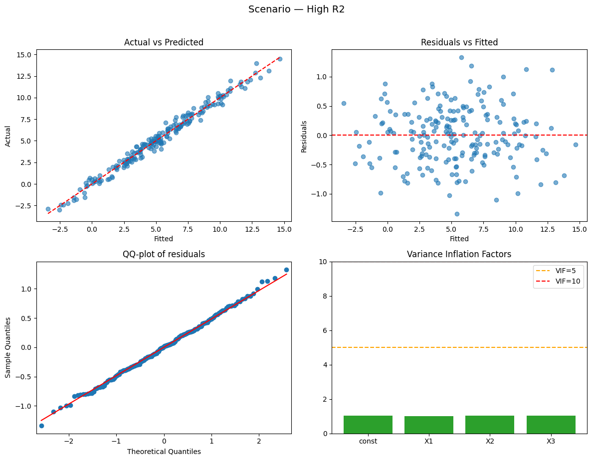
Observations: 200  |  R² = 0.982  (adj R² = 0.982)  —  strong
Overall model: statistically significant  |  F = 3596.20, p = 0.0000

Coefficients:
  - X1: +2.990 (p=0.0000, 95% CI [2.923, 3.057]) — significant
  - X2: -2.042 (p=0.0000, 95% CI [-2.116, -1.968]) — significant
  - X3: +1.487 (p=0.0000, 95% CI [1.419, 1.554]) — significant

VIFs: X1 = 1.01 (low), X2 = 1.04 (low), X3 = 1.04 (low)

Durbin–Watson: ≈ 2 → no clear autocorrelation

Why this happened:
  - High R²: signal (true coefficients) is large relative to noise.


================================================================================
Running scenario: low_r2
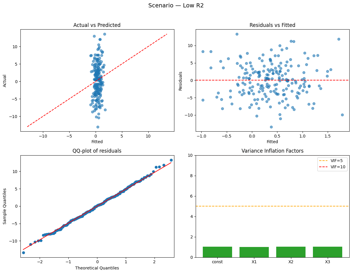
Observations: 200  |  R² = 0.011  (adj R² = -0.004)  —  weak
Overall model: not statistically significant  |  F = 0.74, p = 0.5291

Coefficients:
  - X1: +0.099 (p=0.7725, 95% CI [-0.573, 0.770]) — not significant
  - X2: -0.519 (p=0.1667, 95% CI [-1.257, 0.218]) — not significant
  - X3: -0.082 (p=0.8095, 95% CI [-0.756, 0.591]) — not significant

VIFs: X1 = 1.01 (low), X2 = 1.04 (low), X3 = 1.04 (low)

Durbin–Watson: ≈ 2 → no clear autocorrelation

Why this happened:
  - Low R²: predictors explain little variance because noise dominates.


================================================================================
Running scenario: multicollinearity
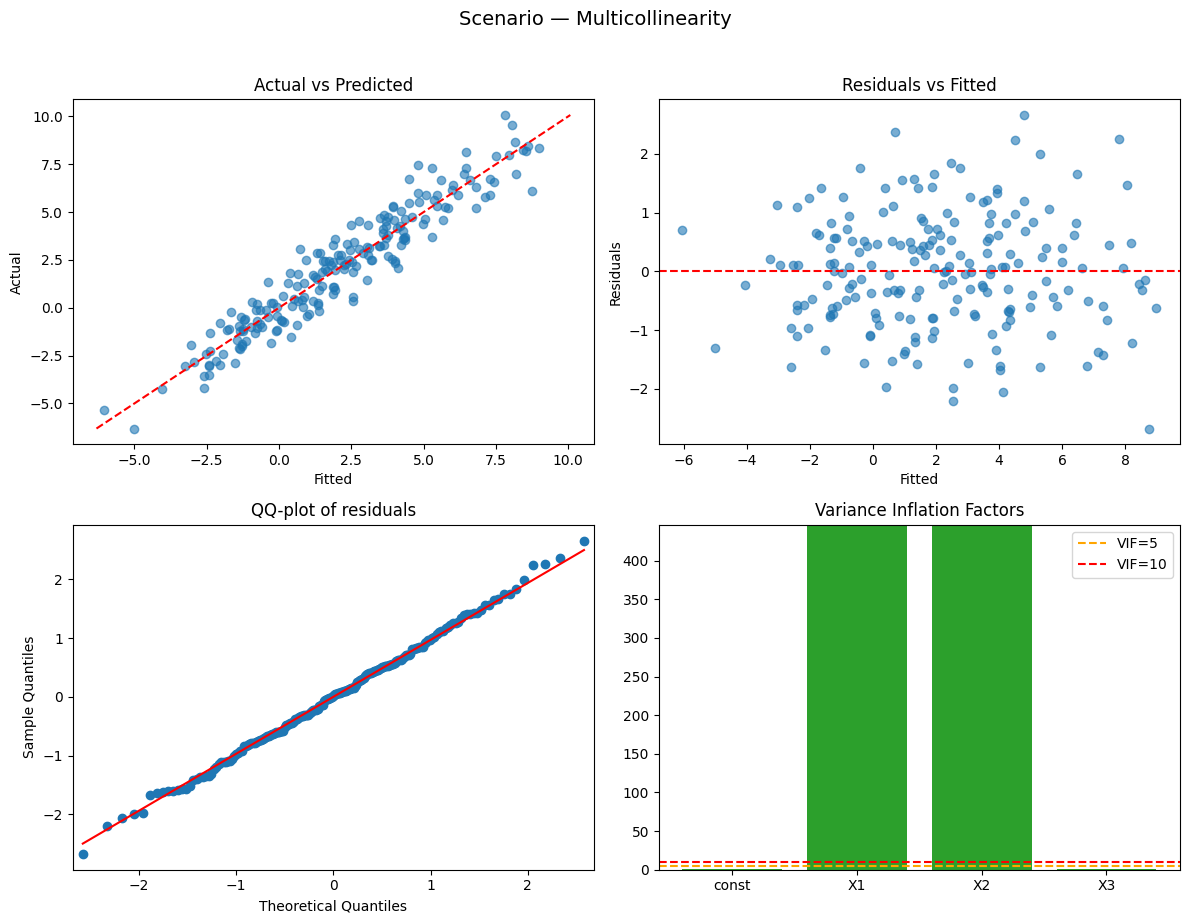
Observations: 200  |  R² = 0.908  (adj R² = 0.907)  —  strong
Overall model: statistically significant  |  F = 646.36, p = 0.0000

Coefficients:
  - X1: +3.073 (p=0.0328, 95% CI [0.255, 5.892]) — significant
  - X2: -0.177 (p=0.9058, 95% CI [-3.129, 2.774]) — not significant
  - X3: -0.526 (p=0.0000, 95% CI [-0.661, -0.392]) — significant

VIFs: X1 = 445.32 (high), X2 = 444.90 (high), X3 = 1.04 (low)

Durbin–Watson: ≈ 2 → no clear autocorrelation

Why this happened:
  - High multicollinearity: similar predictors inflate standard errors (high VIF).


================================================================================
Running scenario: insignificant_predictor
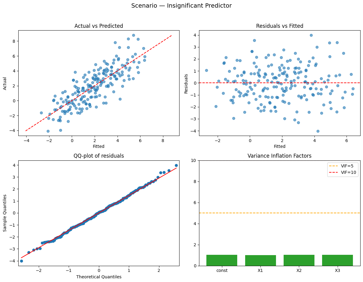
Observations: 200  |  R² = 0.661  (adj R² = 0.656)  —  strong
Overall model: statistically significant  |  F = 127.58, p = 0.0000

Coefficients:
  - X1: +1.970 (p=0.0000, 95% CI [1.768, 2.171]) — significant
  - X2: -0.126 (p=0.2637, 95% CI [-0.347, 0.096]) — not significant
  - X3: +0.460 (p=0.0000, 95% CI [0.258, 0.662]) — significant

VIFs: X1 = 1.01 (low), X2 = 1.04 (low), X3 = 1.04 (low)

Durbin–Watson: ≈ 2 → no clear autocorrelation

Why this happened:
  - One predictor has (near) zero coefficient → will be statistically insignificant.


================================================================================
Running scenario: negative_coefficient
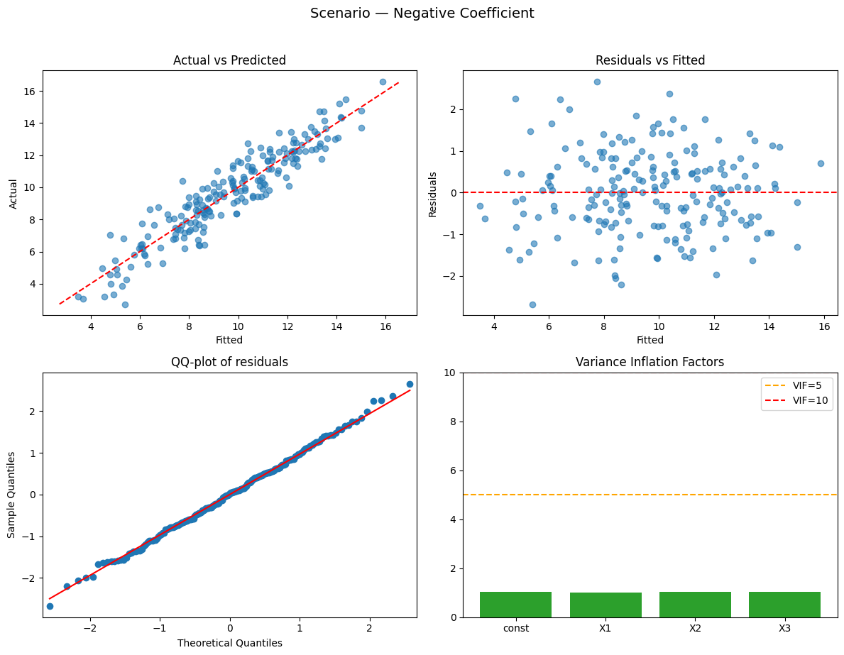
Observations: 200  |  R² = 0.876  (adj R² = 0.874)  —  strong
Overall model: statistically significant  |  F = 460.89, p = 0.0000

Coefficients:
  - X1: -2.520 (p=0.0000, 95% CI [-2.655, -2.386]) — significant
  - X2: +0.416 (p=0.0000, 95% CI [0.269, 0.564]) — significant
  - X3: -0.026 (p=0.6986, 95% CI [-0.161, 0.108]) — not significant

VIFs: X1 = 1.01 (low), X2 = 1.04 (low), X3 = 1.04 (low)

Durbin–Watson: ≈ 2 → no clear autocorrelation

Why this happened:
  - Negative coefficient example — sign is determined by the data-generating process.


================================================================================
Running scenario: autocorrelation
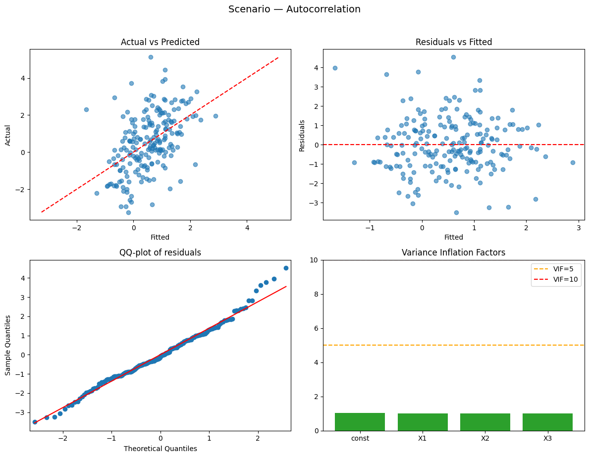
Observations: 200  |  R² = 0.238  (adj R² = 0.227)  —  weak
Overall model: statistically significant  |  F = 20.44, p = 0.0000

Coefficients:
  - X1: +0.588 (p=0.0000, 95% CI [0.394, 0.783]) — significant
  - X2: +0.443 (p=0.0000, 95% CI [0.252, 0.634]) — significant
  - X3: +0.268 (p=0.0113, 95% CI [0.061, 0.474]) — significant

VIFs: X1 = 1.00 (low), X2 = 1.01 (low), X3 = 1.01 (low)

Durbin–Watson: 0.63 → possible positive autocorrelation

Why this happened:
  - Autocorrelated residuals (AR(1)) — Durbin–Watson will be far from 2.


================================================================================
Running scenario: heteroscedasticity
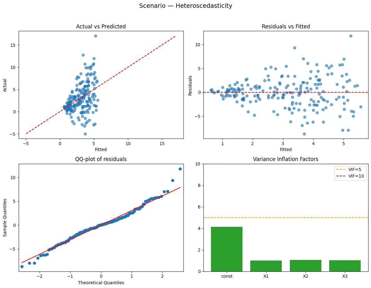
Observations: 200  |  R² = 0.156  (adj R² = 0.143)  —  weak
Overall model: statistically significant  |  F = 12.05, p = 0.0000

Coefficients:
  - X1: +0.461 (p=0.0000, 95% CI [0.308, 0.614]) — significant
  - X2: +0.176 (p=0.4505, 95% CI [-0.283, 0.635]) — not significant
  - X3: +0.145 (p=0.5070, 95% CI [-0.284, 0.573]) — not significant

VIFs: X1 = 1.02 (low), X2 = 1.06 (low), X3 = 1.04 (low)

Durbin–Watson: ≈ 2 → no clear autocorrelation

Why this happened:
  - Heteroscedasticity: residual variance increases with X1 — affects standard errors.


================================================================================
Running scenario: outliers
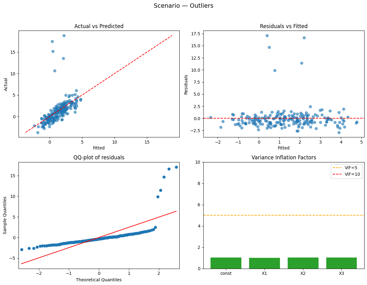
Observations: 200  |  R² = 0.265  (adj R² = 0.254)  —  weak
Overall model: statistically significant  |  F = 23.56, p = 0.0000

Coefficients:
  - X1: +1.452 (p=0.0000, 95% CI [1.110, 1.794]) — significant
  - X2: -0.178 (p=0.3506, 95% CI [-0.554, 0.197]) — not significant
  - X3: -0.017 (p=0.9218, 95% CI [-0.360, 0.326]) — not significant

VIFs: X1 = 1.01 (low), X2 = 1.04 (low), X3 = 1.04 (low)

Durbin–Watson: ≈ 2 → no clear autocorrelation

Why this happened:
  - A few large outliers that can disproportionately affect coefficients and R².