Non-linear & Polynomial Features#
Because not everything in business (or life) is a straight line. 😏
🧠 Why Go Beyond Linear?#
Let’s face it — most real-world business relationships aren’t linear:
Example |
Relationship |
Reality Check |
|---|---|---|
Advertising Spend vs Sales |
“More spend = more sales” |
Until saturation kicks in 💸📉 |
Employee Experience vs Productivity |
“More experience = better output” |
Until burnout 😵 |
Discounts vs Revenue |
“Bigger discounts = higher revenue” |
Until customers expect discounts forever 🫠 |
In short:
Real business curves aren’t straight. So why should our regression lines be?
🎯 The Goal#
We’re still using linear regression — but instead of using X, we’ll also include X², X³, etc.
That gives our model wiggles to fit non-linear patterns.
[ y = \beta_0 + \beta_1 X + \beta_2 X^2 + \beta_3 X^3 + \dots + \varepsilon ]
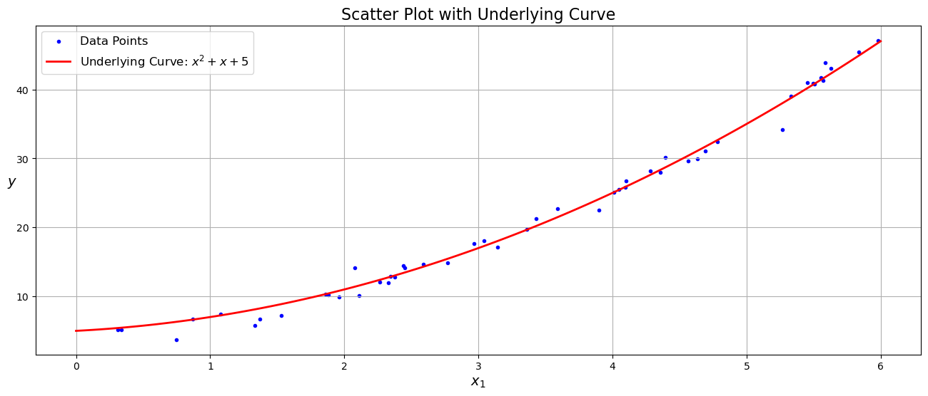
🧩 A Simple Example: Ads vs Sales (Again)#
🎨 Business translation: The red line = your early startup expectations 🚀 The green curve = the reality of scaling with budget constraints 📉📈
🧮 How PolynomialFeatures Works#
When you apply:
If X = [x₁], you get:
Feature |
Formula |
|---|---|
x₀ |
1 (intercept) |
x₁ |
Original feature |
x₁² |
Squared term |
x₁³ |
Cubic term |
Your simple feature becomes a mini feature family — turning “linear regression” into a “non-linear powerhouse.” 💪
💼 Business Analogy#
Imagine your sales vs marketing spend data:
The first few ad dollars give big returns (new awareness 💡)
Then, diminishing returns kick in (everyone’s already seen the ad 😒)
Finally, overspending may even hurt profits (budget wasted 💀)
Polynomial regression captures exactly that:
The rise → plateau → fall pattern that linear models can’t express.
⚠️ Beware of Overfitting#
Polynomial models are like giving your regression model too much artistic freedom: 🎨
Degree 2 = smooth, business-like curve
Degree 5 = chaotic Picasso of your data
💬 Lesson: Don’t let your model hallucinate curves that don’t exist in reality (that’s marketing’s job 😉).
📊 Performance Comparison#
Model |
R² Score |
Interpretation |
|---|---|---|
Linear (Degree 1) |
0.62 |
Basic trend captured |
Polynomial (Degree 2) |
0.88 |
Great fit without overfitting |
Polynomial (Degree 5) |
0.99 (on training) |
🚨 Overfit alert! |
Just because your model fits the training data perfectly doesn’t mean it predicts future business trends. (Ask any crypto investor. 🪙😅)
🧰 Quick Practice: Curve Fitting Yourself#
Task:
Create a dataset for “Price vs Demand” where demand drops exponentially as price increases.
Fit both a linear and a degree 3 polynomial regression.
Visualize both fits and compare performance with R².
Bonus: Add noise and see how overfitting worsens.
(You can run this in JupyterLite, Colab, or download the notebook — whichever fits your caffeine schedule ☕)
🐍 Python Refresher#
If all those NumPy arrays and matrix operations feel like alphabet soup — no worries! 🍜 Check out my other book 👉 Programming for Business It’ll walk you through Python essentials, data handling, and plotting in a fun, business-focused way.
🧭 Recap#
Concept |
Meaning |
|---|---|
Polynomial Features |
Add powers of variables to capture non-linearity |
Degree |
Controls the curve flexibility |
Advantage |
Models complex business relationships |
Risk |
Overfitting if degree is too high |
Best Practice |
Start small (deg=2 or 3), validate on unseen data |
💬 Final Thought#
“Linear regression draws the line. Polynomial regression draws the story behind that line.” 🎭
🔜 Next Up#
🎯 Regularization (Ridge, Lasso, Elastic Net) where we’ll learn how to control overfitting and keep models humble — just like a CFO limits marketing’s budget. 💸🧮
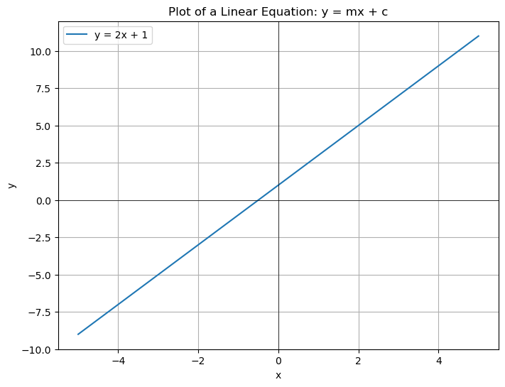
import matplotlib.pyplot as plt
import numpy as np

# Define the slope (m) and y-intercept (c)
m = 2
c = 1

# Generate x values for the line
x = np.linspace(-5, 5, 100)

# Calculate the corresponding y values using the equation y = mx + c
y = m * x + c

# Create the plot
plt.figure(figsize=(8, 6))
plt.plot(x, y, label=f'y = {m}x + {c}')
plt.title('Plot of a Linear Equation: y = mx + c')
plt.xlabel('x')
plt.ylabel('y')
plt.grid(True)
plt.axhline(0, color='black', linewidth=0.5)  # Add x-axis
plt.axvline(0, color='black', linewidth=0.5)  # Add y-axis
plt.legend()
plt.show()
import numpy as np
import matplotlib.pyplot as plt

np.random.seed(50)
m = 50
X = 6 * np.random.rand(m, 1)
y = X ** 2 + X + 5 + np.random.randn(m, 1)  # Adjusted y to be a single column

plt.figure(figsize=(16, 6))  # Increased figure height for better visualization

# Plot the scatter points
plt.scatter(X, y, color="blue", marker=".", label="Data Points")

# Generate points for the curve (without noise)
X_curve = np.linspace(0, 6, 100).reshape(-1, 1)
y_curve = X_curve ** 2 + X_curve + 5

# Plot the underlying curve
plt.plot(X_curve, y_curve, color="red", linestyle="-", linewidth=2, label="Underlying Curve: $x^2 + x + 5$")

plt.xlabel("$x_1$", fontsize=14)
plt.ylabel("$y$", rotation=0, fontsize=14)
plt.title("Scatter Plot with Underlying Curve", fontsize=16)
plt.legend(fontsize=12)
plt.grid(True)
plt.show()
import numpy as np
import matplotlib.pyplot as plt
def polynomial_evaluate(coeffs, x):
return np.polyval(coeffs, x)
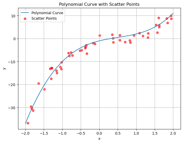
# Define a polynomial: 2x^3 - 3x^2 + 4x - 1
coeffs = [2, -3, 4, -1]
# Evaluate the polynomial at x = 2
x_eval = 2
result = polynomial_evaluate(coeffs, x_eval)
print(f"p({x_eval}) = {result}")
# Plot the polynomial with scatter points
x_curve = np.linspace(-2, 2, 100)
y_curve = polynomial_evaluate(coeffs, x_curve)
# Generate scatter points along the curve with noise
num_points = 50
x_points = np.random.uniform(-2, 2, num_points)
noise_amplitude = 2 # Adjust for the amount of scatter
noise = noise_amplitude * np.random.randn(num_points)
y_points = polynomial_evaluate(coeffs, x_points) + noise
plt.figure(figsize=(8, 6))
plt.plot(x_curve, y_curve, label='Polynomial Curve')
plt.scatter(x_points, y_points, c='red', alpha=0.6, label='Scatter Points')
plt.title("Polynomial Curve with Scatter Points")
plt.xlabel("x")
plt.ylabel("y")
plt.grid(True)
plt.legend()
plt.show()
p(2) = 11
import numpy as np
import matplotlib.pyplot as plt
def polynomial_evaluate(coeffs, x):
return np.polyval(coeffs, x)
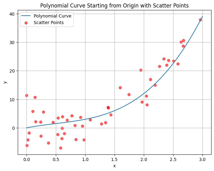
# Define a polynomial: 2x^3 - 3x^2 + 4x
# Removed the -1 to make it pass through origin
coeffs = [2, -3, 4, 0] # Changed the coefficients
# Evaluate the polynomial at x = 2
x_eval = 2
result = polynomial_evaluate(coeffs, x_eval)
print(f"p({x_eval}) = {result}")
# Plot the polynomial and scatter points
x = np.linspace(0, 3, 100) # Adjusted x range to start from 0
y = polynomial_evaluate(coeffs, x)
# Generate scatter points
num_points = 50
x_points = np.random.uniform(0, 3, num_points)
noise_amplitude = 5
noise = noise_amplitude * np.random.randn(num_points)
y_points = polynomial_evaluate(coeffs, x_points) + noise
plt.figure(figsize=(8, 6))
plt.plot(x, y, label='Polynomial Curve')
plt.scatter(x_points, y_points, c='red', alpha=0.6, label='Scatter Points')
plt.title("Polynomial Curve Starting from Origin with Scatter Points")
plt.xlabel("x")
plt.ylabel("y")
plt.grid(True)
plt.legend()
plt.show()
p(2) = 12
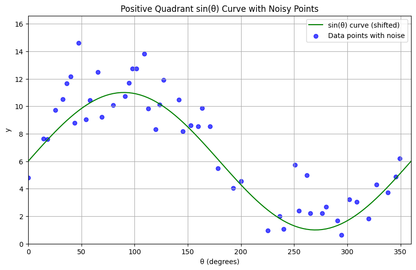
import numpy as np
import matplotlib.pyplot as plt

np.random.seed(42)  # for reproducibility

# Define the range for theta (in degrees)
theta_deg = np.linspace(0, 360, 100)
theta_rad = np.deg2rad(theta_deg)

# Choose between sine or cosine
function_type = "sin"  # You can change this to "cos"

if function_type == "sin":
    y_base = np.sin(theta_rad)
elif function_type == "cos":
    y_base = np.cos(theta_rad)
else:
    raise ValueError("Invalid function_type. Choose 'sin' or 'cos'.")

# Adjust the curve to be in the positive quadrant
# We'll shift and scale the curve
amplitude = 5  # Adjust for the vertical range of the curve
vertical_shift = amplitude + 1 # Shift up so the minimum is above zero
y_base_positive = amplitude * y_base + vertical_shift

# Generate random noise
num_points = 50
random_indices = np.random.choice(len(theta_deg), size=num_points, replace=False)
theta_points_deg = theta_deg[random_indices]
theta_points_rad = np.deg2rad(theta_points_deg)
noise_amplitude = 1.5  # Adjust for the amount of scatter
noise = noise_amplitude * np.random.randn(num_points)

# Calculate the y-coordinates for the scattered points
if function_type == "sin":
    y_points = amplitude * np.sin(theta_points_rad) + vertical_shift + noise
elif function_type == "cos":
    y_points = amplitude * np.cos(theta_points_rad) + vertical_shift + noise

# Ensure all y_points are in the positive quadrant (just a safety measure)
y_points = np.abs(y_points) + 0.5 # Adding a small offset to ensure positivity

# Create the plot
plt.figure(figsize=(10, 6))
plt.plot(theta_deg, y_base_positive, "g-", label=f"{function_type}(θ) curve (shifted)")
plt.scatter(theta_points_deg, y_points, color="blue", alpha=0.7, label="Data points with noise")
plt.xlabel("θ (degrees)")
plt.ylabel("y")
plt.title(f"Positive Quadrant {function_type}(θ) Curve with Noisy Points")
plt.xlim(0, 360)
plt.ylim(0, np.max(y_points) + 2) # Adjust y-axis limits
plt.grid(True)
plt.legend()
plt.show()
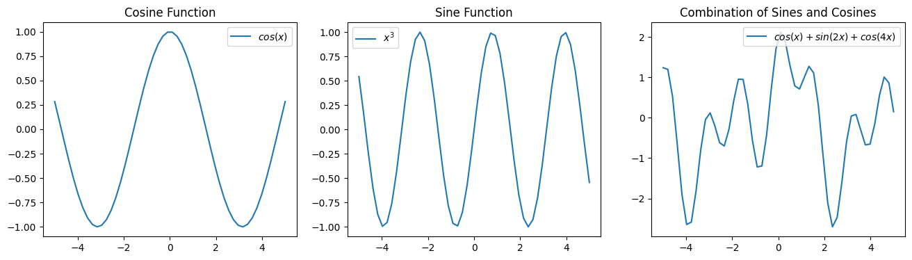
Non-Linear Least Squares#
Ordinary Least Squares can only learn linear relationships in the data. Can we also use it to model more complex relationships?
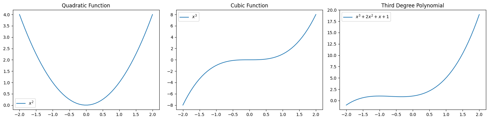
Polynomial Functions#
a polynomial of degree \(p\) is a function of the form $\( a_p x^p + a_{p-1} x^{p-1} + ... + a_{1} x + a_0. \)$
Below are some examples of polynomial functions.
import warnings
import numpy as np
import matplotlib.pyplot as plt

warnings.filterwarnings("ignore")

plt.figure(figsize=(16,4))
x_vars = np.linspace(-2, 2)

plt.subplot(1, 3, 1)
plt.title('Quadratic Function')
plt.plot(x_vars, x_vars**2)
plt.legend(["$x^2$"])

plt.subplot(1, 3, 2)
plt.title('Cubic Function')
plt.plot(x_vars, x_vars**3)
plt.legend(["$x^3$"])

plt.subplot(1, 3, 3)
plt.title('Third Degree Polynomial')
plt.plot(x_vars, x_vars**3 + 2*x_vars**2 + x_vars + 1)
plt.legend(["$x^3 + 2 x^2 + x + 1$"])

plt.tight_layout() # This helps prevent titles from overlapping
plt.show()
import warnings
warnings.filterwarnings("ignore")

plt.figure(figsize=(16,4))
x_vars = np.linspace(-5, 5)

plt.subplot(1, 3, 1)
plt.title('Cosine Function')
plt.plot(x_vars, np.cos(x_vars))
plt.legend(["$cos(x)$"])

plt.subplot(1, 3, 2)
plt.title('Sine Function')
plt.plot(x_vars, np.sin(2*x_vars))
plt.legend(["$x^3$"])

plt.subplot(1, 3, 3)
plt.title('Combination of Sines and Cosines')
plt.plot(x_vars, np.cos(x_vars) + np.sin(2*x_vars) + np.cos(4*x_vars))
plt.legend(["$cos(x) + sin(2x) + cos(4x)$"])
<matplotlib.legend.Legend at 0x10f36a540>
import numpy as np
import matplotlib.pyplot as plt
def generate_polynomial_features(X, degree):
"""Generates polynomial features for a given input array.
Args:
X (np.ndarray): The input array of shape (n_samples,).
degree (int): The degree of the polynomial.
Returns:
np.ndarray: A matrix of shape (n_samples, degree) where each column
represents X raised to the power of (1, 2, ..., degree).
"""
n_samples = X.shape[0]
poly_features = np.empty((n_samples, degree))
for i in range(1, degree + 1):
poly_features[:, i - 1] = X ** i
return poly_features
def fit_polynomial_regression(X_poly, y, learning_rate=0.01, n_iterations=1000):
"""Fits a polynomial regression model using gradient descent.
Args:
X_poly (np.ndarray): The polynomial features of shape (n_samples, degree).
y (np.ndarray): The target values of shape (n_samples,).
learning_rate (float): The learning rate for gradient descent.
n_iterations (int): The number of iterations for gradient descent.
Returns:
np.ndarray: The learned coefficients of the polynomial.
"""
n_samples, n_features = X_poly.shape
# Initialize coefficients with random values
coefficients = np.random.randn(n_features)
# Add a bias term (intercept) to the polynomial features
X_poly = np.concatenate((np.ones((n_samples, 1)), X_poly), axis=1)
coefficients = np.concatenate(([0], coefficients)) # Initialize bias to 0
for _ in range(n_iterations):
# Calculate predictions
y_predicted = np.dot(X_poly, coefficients)
# Calculate the error
error = y_predicted - y
# Calculate gradients
gradients = (1 / n_samples) * np.dot(X_poly.T, error)
# Update coefficients
coefficients = coefficients - learning_rate * gradients
return coefficients
def predict_polynomial(X, coefficients):
"""Predicts values using the learned polynomial regression coefficients.
Args:
X (np.ndarray): The input array for prediction.
coefficients (np.ndarray): The learned coefficients.
Returns:
np.ndarray: The predicted values.
"""
degree = len(coefficients) - 1
X_poly = np.empty((X.shape[0], degree))
for i in range(1, degree + 1):
X_poly[:, i - 1] = X ** i
# Add bias term
X_poly = np.concatenate((np.ones((X.shape[0], 1)), X_poly), axis=1)
return np.dot(X_poly, coefficients)
np.random.seed(42)
n_samples = 30
X = np.sort(np.random.rand(n_samples))
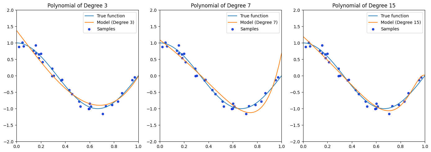
true_fn = lambda x: np.cos(1.5 * np.pi * x)
y = true_fn(X) + np.random.normal(0, 0.1, n_samples)
degrees = [3, 7, 15]
plt.figure(figsize=(14, 5))
X_test = np.linspace(0, 1, 100)
for i, degree in enumerate(degrees):
ax = plt.subplot(1, len(degrees), i + 1)
# Generate polynomial features
X_poly = generate_polynomial_features(X, degree)
# Fit the polynomial regression model
coefficients = fit_polynomial_regression(X_poly, y, learning_rate=0.1, n_iterations=5000)
# Predict on the test data
X_test_poly = generate_polynomial_features(X_test, degree)
y_predicted = predict_polynomial(X_test, coefficients)
# Plotting
ax.plot(X_test, true_fn(X_test), label="True function")
ax.plot(X_test, y_predicted, label=f"Model (Degree {degree})")
ax.scatter(X, y, edgecolor='b', s=20, label="Samples")
ax.set_xlim((0, 1))
ax.set_ylim((-2, 2))
ax.legend(loc="best")
ax.set_title(f"Polynomial of Degree {degree}")
plt.tight_layout()
plt.show()
Absolutely! Let’s dive into the intuition behind generating polynomial features.
Imagine you have a set of data points, and when you plot them, they clearly don’t fall on a straight line. Instead, they seem to follow a curve.
The Limitation of Linear Regression:
Linear regression, at its core, tries to find the best straight line that fits your data. It models the relationship between your input features (\(X\)) and your output (\(y\)) as:
where \(\beta_0, \beta_1, ..., \beta_n\) are the coefficients it learns. This equation represents a hyperplane (a line in 2D, a plane in 3D, and so on). If the underlying relationship in your data is not linear, a straight line will likely do a poor job of capturing the pattern.
The Idea of Polynomial Regression:
Polynomial regression comes into play when you suspect a non-linear relationship between your variables. The fundamental idea is to transform your original input features into a higher-dimensional space by adding polynomial terms.
How it Works (Intuition with a Single Feature):
Let’s say you have a single input feature, \(x\), and your data looks like a parabola (a U-shape). A simple linear model would be \(y \approx \beta_0 + \beta_1 x\). This can only fit a straight line.
To capture the curvature, we can introduce a new feature: \(x^2\). Now, our model becomes:
Notice that although the model itself is still linear in terms of the coefficients (\(\beta_0, \beta_1, \beta_2\)), it can now represent a parabolic curve because the input \(x\) is transformed non-linearly.
Visualizing the Transformation:
Think of it this way:
Original Space: You have your data points in a 2D space with axes \(x\) and \(y\). The relationship is curved.
Feature Transformation: You create a new “feature” by squaring the original \(x\) values. Now, for each data point \((x_i, y_i)\), you can think of it as existing in a new 3D space with axes \(x\), \(x^2\), and \(y\).
Linear Regression in the Transformed Space: In this new 3D space, the relationship between \(x\), \(x^2\), and \(y\) might be linear. Our linear regression algorithm finds a plane that best fits these points in the 3D space: \(y \approx \beta_0 \cdot 1 + \beta_1 \cdot x + \beta_2 \cdot x^2\).
Mapping Back to the Original Space: When you plot the resulting equation \(y = \beta_0 + \beta_1 x + \beta_2 x^2\) in the original 2D space (with axes \(x\) and \(y\)), you get a parabola!
Generalizing to Higher Degrees:
You can extend this idea to even higher degree polynomials. For a degree-\(d\) polynomial with a single feature \(x\), you would generate features \(x^1, x^2, x^3, ..., x^d\). Your model would then be:
By including these higher-order terms, the model gains the flexibility to fit more complex curves in your data.
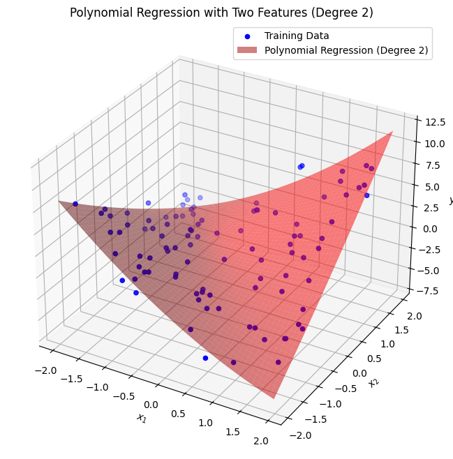
With Multiple Features:
If you have multiple input features (\(x_1, x_2, ...\)), generating polynomial features involves creating terms that are products of the original features raised to various powers (up to the specified degree). For example, for degree 2 with two features, you’d have terms like:
\(x_1\)
\(x_2\)
\(x_1^2\)
\(x_2^2\)
\(x_1 x_2\)
This allows the model to capture not only the individual non-linear effects of each feature but also their interactions.
In essence, generating polynomial features allows us to use the power of linear models to fit non-linear relationships by transforming the input data into a higher-dimensional space where the relationship might be linear. The linear regression algorithm then learns the coefficients in this transformed space, which, when mapped back to the original feature space, results in a polynomial curve.
Think of it like bending a straight ruler. A straight ruler can only fit straight lines. But if you could somehow manipulate your data so that the relationship appears straight in a different “bent” space, then a straight ruler (linear regression) could fit it perfectly in that space. When you unbend the space back to normal, the straight line becomes a curve. Polynomial feature generation is a way to mathematically “bend” the space of your features.
import numpy as np
import matplotlib.pyplot as plt
from sklearn.preprocessing import PolynomialFeatures
from sklearn.linear_model import LinearRegression
from mpl_toolkits.mplot3d import Axes3D  # Import for 3D plotting

# Generate sample data with two features
np.random.seed(42)
m = 100
X_multi = np.random.rand(m, 2) * 4 - 2  # Features between -2 and 2
y_multi = 0.5 * X_multi[:, 0]**2 + 0.3 * X_multi[:, 1]**3 + 2 * X_multi[:, 0] * X_multi[:, 1] + np.random.randn(m)

# Fit a polynomial regression model (degree 2 for simplicity in visualization)
degree_multi = 2
poly_features_multi = PolynomialFeatures(degree=degree_multi, include_bias=False)
X_poly_multi = poly_features_multi.fit_transform(X_multi)
lin_reg_multi = LinearRegression()
lin_reg_multi.fit(X_poly_multi, y_multi)

# Create a grid of x1 and x2 values for plotting the prediction surface
x1_surf, x2_surf = np.meshgrid(np.linspace(X_multi[:, 0].min(), X_multi[:, 0].max(), 50),
                               np.linspace(X_multi[:, 1].min(), X_multi[:, 1].max(), 50))

# Create the polynomial features for the grid
X_surf = np.c_[x1_surf.ravel(), x2_surf.ravel()]
X_poly_surf = poly_features_multi.transform(X_surf)

# Predict the y values for the grid
y_surf = lin_reg_multi.predict(X_poly_surf).reshape(x1_surf.shape)

# Create the 3D plot
fig = plt.figure(figsize=(12, 8))
ax = fig.add_subplot(111, projection='3d')

# Scatter plot of the data points
ax.scatter(X_multi[:, 0], X_multi[:, 1], y_multi, c='blue', marker='o', label='Training Data')

# Plot the regression surface
ax.plot_surface(x1_surf, x2_surf, y_surf, color='red', alpha=0.5, label=f'Polynomial Regression (Degree {degree_multi})')

ax.set_xlabel('$x_1$')
ax.set_ylabel('$x_2$')
ax.set_zlabel('$y$')
ax.set_title(f'Polynomial Regression with Two Features (Degree {degree_multi})')
ax.legend()
plt.show()
import numpy as np
import matplotlib.pyplot as plt
from sklearn.preprocessing import PolynomialFeatures
from sklearn.linear_model import LinearRegression
from mpl_toolkits.mplot3d import Axes3D
import matplotlib.animation as animation

# ... (rest of your data generation and fitting code) ...

fig = plt.figure(figsize=(12, 8))
ax = fig.add_subplot(111, projection='3d')
ax.scatter(X_multi[:, 0], X_multi[:, 1], y_multi, c='blue', marker='o', label='Training Data')
ax.plot_surface(x1_surf, x2_surf, y_surf, color='red', alpha=0.5, label=f'Polynomial Regression (Degree {degree_multi})')
ax.set_xlabel('$x_1$')
ax.set_ylabel('$x_2$')
ax.set_zlabel('$y$')
ax.set_title(f'Polynomial Regression with Two Features (Degree {degree_multi})')
ax.legend()

def rotate(angle):
    ax.view_init(elev=20, azim=angle)

ani = animation.FuncAnimation(fig, rotate, frames=np.arange(0, 360, 2), interval=50)

plt.show()

# To save the animation (requires a writer like 'ffmpeg' or ' PillowWriter'):
ani.save('rotation.gif', writer='pillow')
from IPython.display import Image
Image(filename="rotation.gif")
import numpy as np
from scipy.linalg import lstsq
from sklearn.preprocessing import StandardScaler, PolynomialFeatures
from sklearn.pipeline import Pipeline
class PolynomialRegressionSVD:
def __init__(self, degree=2):
self.degree = degree
self.poly = PolynomialFeatures(degree=degree, include_bias=True)
self.scaler = StandardScaler()
def fit(self, X, y):
# Generate polynomial features
X_poly = self.poly.fit_transform(X)
# Scale features (except bias term)
if X_poly.shape[1] > 1: # Only scale if there are features beyond the bias
X_poly[:, 1:] = self.scaler.fit_transform(X_poly[:, 1:])
# Solve using SVD (via scipy.linalg.lstsq)
self.coef_, _, _, _ = lstsq(X_poly, y)
return self
def predict(self, X):
X_poly = self.poly.transform(X)
if X_poly.shape[1] > 1:
X_poly[:, 1:] = self.scaler.transform(X_poly[:, 1:])
return X_poly @ self.coef_
# Example usage
if __name__ == "__main__":
import matplotlib.pyplot as plt
# Generate sample data
np.random.seed(42)
X = 6 * np.random.rand(100, 1).astype(np.float64) - 3
y = (0.5 * X**2 + X + 2 + np.random.randn(100, 1)).astype(np.float64)
# Test high-degree polynomial
model = PolynomialRegressionSVD(degree=10)
model.fit(X, y)
# Plot results
plt.figure(figsize=(10, 6))
X_new = np.linspace(-3, 3, 100).reshape(-1, 1)
y_pred = model.predict(X_new)
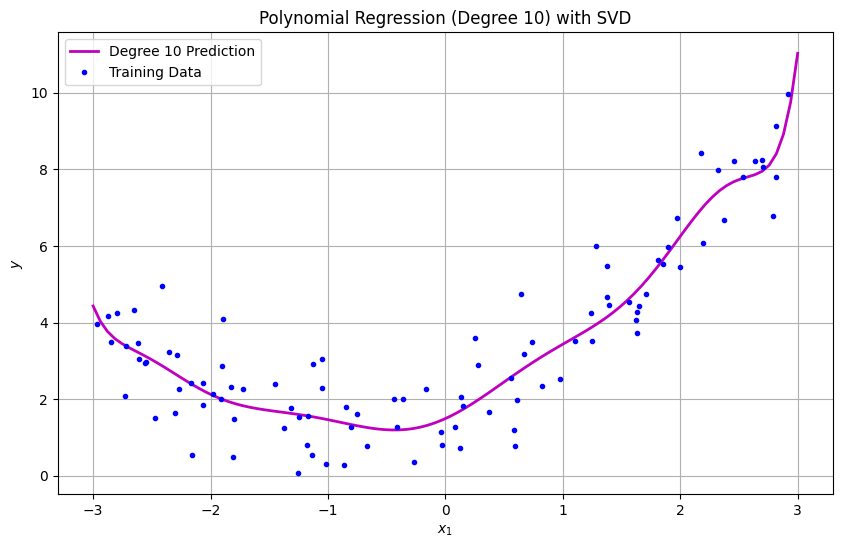
plt.plot(X_new, y_pred, "m-", linewidth=2, label="Degree 10 Prediction")
plt.plot(X, y, "b.", label="Training Data")
plt.xlabel("$x_1$")
plt.ylabel("$y$")
plt.title("Polynomial Regression (Degree 10) with SVD")
plt.legend()
plt.grid(True)
plt.show()
/var/folders/93/7lt42x5j7m39kz7wxbcghvrm0000gn/T/ipykernel_1061/1992350972.py:29: RuntimeWarning: divide by zero encountered in matmul
  return X_poly @ self.coef_
/var/folders/93/7lt42x5j7m39kz7wxbcghvrm0000gn/T/ipykernel_1061/1992350972.py:29: RuntimeWarning: overflow encountered in matmul
  return X_poly @ self.coef_
/var/folders/93/7lt42x5j7m39kz7wxbcghvrm0000gn/T/ipykernel_1061/1992350972.py:29: RuntimeWarning: invalid value encountered in matmul
  return X_poly @ self.coef_
import numpy as np
import matplotlib.pyplot as plt
from sklearn.preprocessing import StandardScaler
from sklearn.linear_model import LinearRegression
from sklearn.pipeline import make_pipeline
from sklearn.preprocessing import PolynomialFeatures
# --- Polynomial Features with a Single Feature ---
print("\n--- Polynomial Features with a Single Feature ---")
# Sample data with a single feature
np.random.seed(42)
m = 100
X = 6 * np.random.rand(100, 1).astype(np.float64) - 3
y = (0.5 * X**2 + X + 2 + np.random.randn(100, 1)).astype(np.float64)
# Let's explore polynomial features of different degrees for this single feature
degrees_single = [1, 2, 3]
feature_names_single = ["x"]
for degree in degrees_single:
poly_features = PolynomialFeatures(degree=degree, include_bias=False)
X_poly = poly_features.fit_transform(X)
print(f"\nDegree: {degree}")
print("Original features (first 5 samples):\n", X[:5])
print("Polynomial features (first 5 samples):\n", X_poly[:5])
print("Feature names after transformation:", poly_features.get_feature_names_out(feature_names_single))
# Plotting the results of polynomial regression with a single feature
plt.figure(figsize=(10, 6))
X_new_single = np.linspace(-3, 3, 100).reshape(-1, 1)
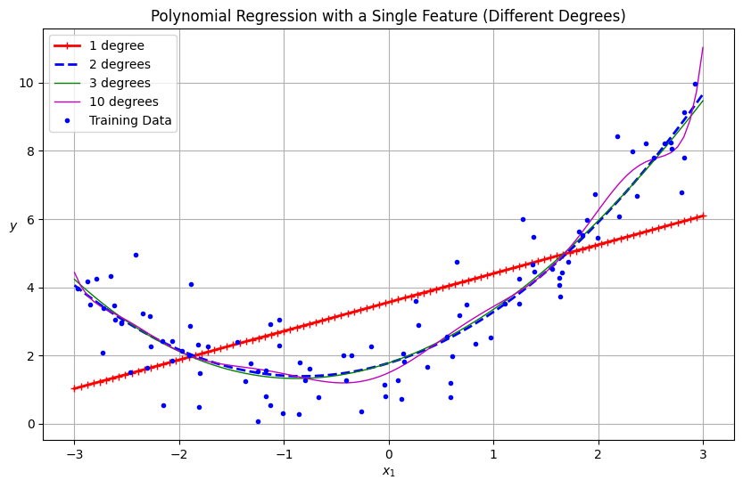
for style, width, degree in (("r-+", 2, 1), ("b--", 2, 2), ("g-", 1, 3), ("m-", 1, 10)):
polybig_features = PolynomialFeatures(degree=degree, include_bias=False)
std_scaler = StandardScaler()
lin_reg = LinearRegression()
polynomial_regression = make_pipeline(polybig_features, std_scaler, lin_reg)
polynomial_regression.fit(X, y)
y_newbig = polynomial_regression.predict(X_new_single)
label = f"{degree} degree{'s' if degree > 1 else ''}"
plt.plot(X_new_single, y_newbig, style, label=label, linewidth=width)
plt.plot(X, y, "b.", linewidth=3, label="Training Data")
plt.legend(loc="upper left")
plt.xlabel("$x_1$")
plt.ylabel("$y$", rotation=0)
plt.title("Polynomial Regression with a Single Feature (Different Degrees)")
plt.grid(True)
plt.show()
# --- Polynomial Features with Multiple Features ---
print("\n--- Polynomial Features with Multiple Features ---")
# Sample data with two features
np.random.seed(42)
m = 100
X_multi = np.random.rand(m, 2) * 4 - 2 # Features between -2 and 2
y_multi = 0.5 * X_multi[:, 0]**2 + 0.3 * X_multi[:, 1]**3 + 2 * X_multi[:, 0] * X_multi[:, 1] + np.random.randn(m)
# Let's explore polynomial features of degree 2 for these two features
degree_multi = 2
poly_features_multi = PolynomialFeatures(degree=degree_multi, include_bias=False)
X_poly_multi = poly_features_multi.fit_transform(X_multi)
feature_names_multi = ["x1", "x2"]
print(f"\nDegree: {degree_multi}")
print("Original features (first 5 samples):\n", X_multi[:5])
print("Polynomial features (first 5 samples):\n", X_poly_multi[:5])
print("Feature names after transformation:", poly_features_multi.get_feature_names_out(feature_names_multi))
# To visualize the regression with multiple features, we'd typically need a 3D plot.
# However, let's focus on understanding the feature transformation here.
# Example of how the features are generated for degree 2 with two original features (x1, x2):
# For degree 2, the features generated are:
# [x1, x2, x1^2, x1 x2, x2^2]
# Let's look at one sample to illustrate:
sample = X_multi[0]
print(f"\nExample for a single data point: {sample}")
transformed_sample = poly_features_multi.transform(sample.reshape(1, -1))
print(f"Transformed features (degree {degree_multi}): {transformed_sample}")
# These correspond to: [x1, x2, x1^2, x1*x2, x2^2]
# --- Visualizing Polynomial Regression with Two Features (Conceptual - Hard to plot directly in 2D) ---
# To visualize this properly, you would need a 3D scatter plot for the data points
# and a 3D surface for the regression plane (in the transformed space, which maps
# back to a more complex surface in the original x1-x2 space).
# The core idea remains: PolynomialFeatures expands the feature space, allowing a
# linear model to fit non-linear relationships in the original feature space.
--- Polynomial Features with a Single Feature ---

Degree: 1
Original features (first 5 samples):
 [[-0.75275929]
 [ 2.70428584]
 [ 1.39196365]
 [ 0.59195091]
 [-2.06388816]]
Polynomial features (first 5 samples):
 [[-0.75275929]
 [ 2.70428584]
 [ 1.39196365]
 [ 0.59195091]
 [-2.06388816]]
Feature names after transformation: ['x']

Degree: 2
Original features (first 5 samples):
 [[-0.75275929]
 [ 2.70428584]
 [ 1.39196365]
 [ 0.59195091]
 [-2.06388816]]
Polynomial features (first 5 samples):
 [[-0.75275929  0.56664654]
 [ 2.70428584  7.3131619 ]
 [ 1.39196365  1.93756281]
 [ 0.59195091  0.35040587]
 [-2.06388816  4.25963433]]
Feature names after transformation: ['x' 'x^2']

Degree: 3
Original features (first 5 samples):
 [[-0.75275929]
 [ 2.70428584]
 [ 1.39196365]
 [ 0.59195091]
 [-2.06388816]]
Polynomial features (first 5 samples):
 [[-0.75275929  0.56664654 -0.42654845]
 [ 2.70428584  7.3131619  19.77688015]
 [ 1.39196365  1.93756281  2.697017  ]
 [ 0.59195091  0.35040587  0.20742307]
 [-2.06388816  4.25963433 -8.79140884]]
Feature names after transformation: ['x' 'x^2' 'x^3']
--- Polynomial Features with Multiple Features ---

Degree: 2
Original features (first 5 samples):
 [[-0.50183952  1.80285723]
 [ 0.92797577  0.39463394]
 [-1.37592544 -1.37602192]
 [-1.76766555  1.46470458]
 [ 0.40446005  0.83229031]]
Polynomial features (first 5 samples):
 [[-0.50183952  1.80285723  0.25184291 -0.90474501  3.25029418]
 [ 0.92797577  0.39463394  0.86113902  0.36621073  0.15573594]
 [-1.37592544 -1.37602192  1.89317081  1.89330356  1.89343632]
 [-1.76766555  1.46470458  3.1246415  -2.58910783  2.14535952]
 [ 0.40446005  0.83229031  0.16358793  0.33662818  0.69270716]]
Feature names after transformation: ['x1' 'x2' 'x1^2' 'x1 x2' 'x2^2']

Example for a single data point: [-0.50183952  1.80285723]
Transformed features (degree 2): [[-0.50183952  1.80285723  0.25184291 -0.90474501  3.25029418]]
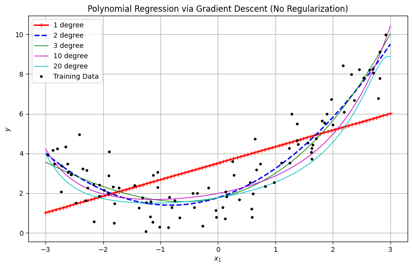
import numpy as np
import matplotlib.pyplot as plt

class PolynomialRegressionGD:
    def __init__(self, degree, learning_rate=1e-3, n_iter=10000, tol=1e-4):
        self.degree = degree
        self.learning_rate = learning_rate
        self.n_iter = n_iter
        self.tol = tol  # Stopping tolerance

    def _polynomial_features(self, X):
        """Generate polynomial features with better numerical stability."""
        features = [np.ones((X.shape[0], 1))]  # Start with bias term
        for d in range(1, self.degree + 1):
            features.append(X ** d)
        return np.hstack(features)

    def _standard_scale(self, X):
        """Standard scaling (mean=0, std=1) with numerical safeguards."""
        self.mean_ = X.mean(axis=0)
        self.std_ = X.std(axis=0)
        # Avoid division by zero and maintain numerical stability
        self.std_[self.std_ < 1e-8] = 1.0  # Threshold for small std dev
        return (X - self.mean_) / self.std_

    def fit(self, X, y):
        # Generate polynomial features (includes bias term)
        X_poly = self._polynomial_features(X)

        # Scale features (excluding bias term)
        X_poly[:, 1:] = self._standard_scale(X_poly[:, 1:])

        m = X_poly.shape[0]
        self.theta = np.zeros((X_poly.shape[1], 1), dtype=np.float64)

        prev_loss = np.inf
        for i in range(self.n_iter):
            # Predictions and error (with numerical safeguards)
            y_pred = np.clip(X_poly @ self.theta, -1e100, 1e100)
            error = y_pred - y

            # Calculate MSE loss only (no regularization)
            loss = (error.T @ error) / m

            # Check for convergence
            if abs(prev_loss - loss.item()) < self.tol:
                break
            prev_loss = loss.item()

            # Calculate gradients (no regularization terms)
            gradients = (2 / m) * X_poly.T @ error

            # Adaptive learning rate for stability
            effective_lr = self.learning_rate / (1 + 0.001 * i)
            self.theta -= effective_lr * gradients

    def predict(self, X):
        X_poly = self._polynomial_features(X)
        X_poly[:, 1:] = (X_poly[:, 1:] - self.mean_) / self.std_
        return np.clip(X_poly @ self.theta, -1e100, 1e100)  # Numerical safeguard

# Generate data
np.random.seed(42)
X = 6 * np.random.rand(100, 1).astype(np.float64) - 3
y = (0.5 * X**2 + X + 2 + np.random.randn(100, 1)).astype(np.float64)

# Plotting
plt.figure(figsize=(10, 6))
X_new = np.linspace(-3, 3, 100).reshape(-1, 1).astype(np.float64)

for style, width, degree, lr in [
    ("r-+", 2, 1, 0.01),
    ("b--", 2, 2, 0.01),
    ("g-", 1, 3, 0.005),
    ("m-", 1, 10, 0.001),
    ("c-", 1, 20, 0.0005)
]:
    model = PolynomialRegressionGD(degree=degree, learning_rate=lr, n_iter=20000)
    model.fit(X, y)
    y_pred = model.predict(X_new)
    plt.plot(X_new, y_pred, style, linewidth=width, label=f"{degree} degree")

plt.plot(X, y, "k.", label="Training Data")
plt.xlabel("$x_1$")
plt.ylabel("$y$")
plt.title("Polynomial Regression via Gradient Descent (No Regularization)")
plt.legend()
plt.grid(True)
plt.show()
/var/folders/93/7lt42x5j7m39kz7wxbcghvrm0000gn/T/ipykernel_1061/2382199848.py:39: RuntimeWarning: divide by zero encountered in matmul
  y_pred = np.clip(X_poly @ self.theta, -1e100, 1e100)
/var/folders/93/7lt42x5j7m39kz7wxbcghvrm0000gn/T/ipykernel_1061/2382199848.py:39: RuntimeWarning: overflow encountered in matmul
  y_pred = np.clip(X_poly @ self.theta, -1e100, 1e100)
/var/folders/93/7lt42x5j7m39kz7wxbcghvrm0000gn/T/ipykernel_1061/2382199848.py:39: RuntimeWarning: invalid value encountered in matmul
  y_pred = np.clip(X_poly @ self.theta, -1e100, 1e100)
/var/folders/93/7lt42x5j7m39kz7wxbcghvrm0000gn/T/ipykernel_1061/2382199848.py:51: RuntimeWarning: divide by zero encountered in matmul
  gradients = (2 / m) * X_poly.T @ error
/var/folders/93/7lt42x5j7m39kz7wxbcghvrm0000gn/T/ipykernel_1061/2382199848.py:51: RuntimeWarning: overflow encountered in matmul
  gradients = (2 / m) * X_poly.T @ error
/var/folders/93/7lt42x5j7m39kz7wxbcghvrm0000gn/T/ipykernel_1061/2382199848.py:51: RuntimeWarning: invalid value encountered in matmul
  gradients = (2 / m) * X_poly.T @ error
/var/folders/93/7lt42x5j7m39kz7wxbcghvrm0000gn/T/ipykernel_1061/2382199848.py:60: RuntimeWarning: divide by zero encountered in matmul
  return np.clip(X_poly @ self.theta, -1e100, 1e100)  # Numerical safeguard
/var/folders/93/7lt42x5j7m39kz7wxbcghvrm0000gn/T/ipykernel_1061/2382199848.py:60: RuntimeWarning: overflow encountered in matmul
  return np.clip(X_poly @ self.theta, -1e100, 1e100)  # Numerical safeguard
/var/folders/93/7lt42x5j7m39kz7wxbcghvrm0000gn/T/ipykernel_1061/2382199848.py:60: RuntimeWarning: invalid value encountered in matmul
  return np.clip(X_poly @ self.theta, -1e100, 1e100)  # Numerical safeguard
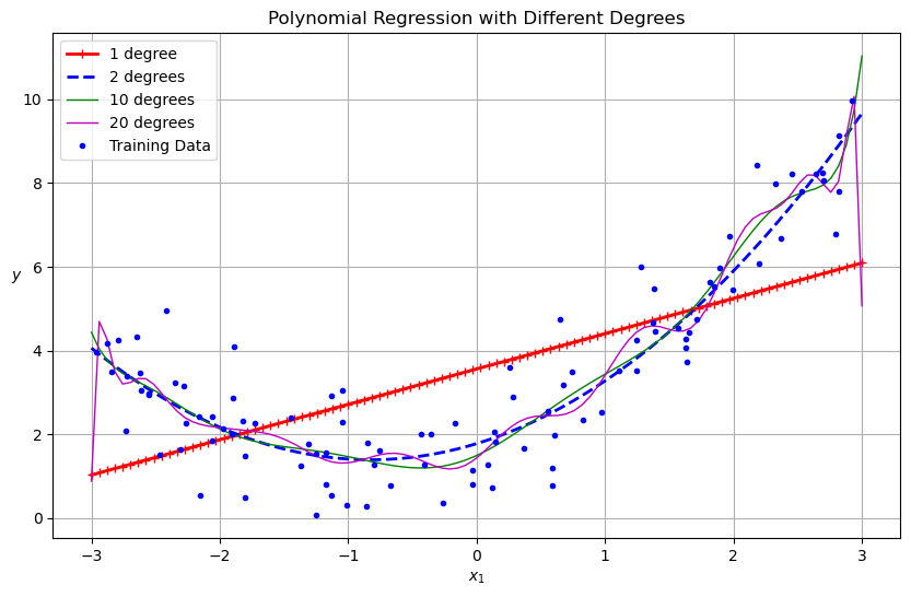
from sklearn.preprocessing import StandardScaler
from sklearn.pipeline import make_pipeline
from sklearn.preprocessing import PolynomialFeatures
from sklearn.linear_model import LinearRegression
import numpy as np
import matplotlib.pyplot as plt

# Generate some sample data for demonstration
np.random.seed(42)
m = 100
X = 6 * np.random.rand(m, 1) - 3
y = 0.5 * X**2 + X + 2 + np.random.randn(m, 1)

# Create data for plotting the predictions
X_new = np.linspace(-3, 3, 100).reshape(-1, 1)

plt.figure(figsize=(10, 6))

for style, width, degree in (("r-+", 2, 1), ("b--", 2, 2), ("g-", 1, 10), ("m", 1, 20)):
    polybig_features = PolynomialFeatures(degree=degree, include_bias=False)
    std_scaler = StandardScaler()
    lin_reg = LinearRegression()
    polynomial_regression = make_pipeline(polybig_features, std_scaler, lin_reg)
    polynomial_regression.fit(X, y)
    y_newbig = polynomial_regression.predict(X_new)
    label = f"{degree} degree{'s' if degree > 1 else ''}"
    plt.plot(X_new, y_newbig, style, label=label, linewidth=width)

plt.plot(X, y, "b.", linewidth=3, label="Training Data")
plt.legend(loc="upper left")
plt.xlabel("$x_1$")
plt.ylabel("$y$", rotation=0)
plt.title("Polynomial Regression with Different Degrees")
plt.grid(True)
plt.show()
References of github
cornell-cs5785-2024-applied-ml
girafe-ai/ml-course
ageron/handson-ml3
maykulkarni/Machine-Learning-Notebooks
# Your code here