Calculus Essentials

Calculus Essentials#

Welcome to Calculus Essentials — the chapter where your ML models finally learn how to learn. Don’t worry — we’re not here to prove theorems. We’re here to explain why your model behaves like an over-caffeinated intern: it keeps making mistakes, learning from them, and slowly improving. ☕🤖

🧠 Why Calculus Matters in ML#

In business terms:

Calculus helps your model minimize regret (also known as “loss”).

It’s the math of change and improvement — used by machine learning algorithms to adjust parameters, reduce errors, and get better at predictions.

Think of it as the “performance review” process for algorithms.

Concept	What It Means in ML	Business Analogy
Derivative	Measures how much something changes	“If ad spend goes up slightly, how does revenue change?”
Gradient	Multi-dimensional derivative	“What’s the direction to move to improve profits?”
Optimization	Using calculus to find the best outcome	“Find the marketing budget that maximizes ROI.”

💡 The Idea in One Sentence#

Machine Learning = Data + Calculus + Patience.

Every training loop goes something like this:

Make a prediction (it’s probably wrong 🙃)
Measure how wrong (loss function)
Use calculus (gradient) to adjust parameters
Try again, but smarter

And that’s gradient descent — the backbone of all modern ML.

⚙️ Meet the Star: The Derivative#

The derivative tells us how fast something changes.

[ \frac{d}{dx}f(x) ]

means “how much does ( f(x) ) change if we nudge ( x ) a little?”

If ( f(x) ) = revenue and ( x ) = ad spend:

[ \frac{d}{dx}f(x) \Rightarrow \text{‘How much does revenue change if we increase ads slightly?’} ]

That’s business calculus — not rocket science. 🚀

🏔️ Finding the Sweet Spot (Minima)#

Imagine your model’s “error” as a landscape of hills and valleys. Your goal? Find the lowest point — the minimum loss.

🏔️ Too high → bad predictions
🕳️ Lowest valley → best model parameters

Gradient descent is your model walking downhill — step by step — until it reaches that sweet spot.

[ \theta = \theta - \eta \cdot \frac{d}{d\theta}L(\theta) ]

Where:

( \theta ) = model parameters
( L(\theta) ) = loss (sadness level)
( \eta ) = learning rate (coffee intake per iteration ☕)

🧩 Practice Corner #1: “Find the Direction”#

Suppose your model’s loss is shaped like a hill: [ L(w) = (w - 3)^2 ]

You start at ( w = 0 ). The slope is:

[ \frac{dL}{dw} = 2(w - 3) ]

At ( w = 0 ): slope = -6 → negative means “go right.” The model learns to move toward ( w = 3 ) — where loss is minimum.

✅ Key Idea: The sign of the derivative tells your model which direction to move. That’s literally “learning” in one line of math.

💬 Common Calculus Concepts in ML#

Symbol	Name	ML Role	Business Analogy
( \frac{d}{dx} )	Derivative	Change in one variable	How revenue reacts to marketing spend
( \nabla L )	Gradient	Multi-variable slope	Direction of steepest improvement
( \eta )	Learning Rate	Step size	“How aggressive should we change strategy?”
( L(\theta) )	Loss Function	Model’s total error	“How wrong are we?”
( \min L(\theta) )	Optimization	Goal of training	“Find the best possible outcome.”

🧩 Practice Corner #2: “Business Gradient Descent”#

Your model predicts sales with one parameter — price. It’s currently too high, and customers are leaving.

What should the model do?

Observation	Derivative Sign	Adjustment
Price ↑ → Sales ↓	Negative	Move price down
Price ↓ → Sales ↑	Positive	Move price up

💡 Models don’t know “cheap” or “expensive.” They just see gradients — mathematical hints toward better business outcomes.

⚖️ Business Translation: “Gradient Descent in Real Life”#

Let’s compare:

Model Training	Business Analogy
Model makes bad prediction	Employee makes mistake
Calculate loss	You review KPIs
Compute gradient	You identify what went wrong
Update weights	Employee learns and improves
Repeat	Continuous improvement cycle

Yes — your ML model is basically a self-correcting employee that never sleeps and works for free. 🤖💼

🎓 Quick Recap#

✅ Derivatives measure change ✅ Gradients tell direction ✅ Learning rate controls speed ✅ Loss function defines goal ✅ Gradient descent = how models learn from mistakes

🧠 Bonus: The Secret Behind Backpropagation#

If you’ve heard “backpropagation” in neural networks — that’s just calculus playing catch-up.

The model:

Makes a forward pass (predicts)
Measures error (loss)
Uses calculus (chain rule) to assign blame
Updates weights accordingly

In other words:

Backprop = Calculus + Accountability.

🧩 Practice Corner #3: “Check Your Intuition”#

Question	Your Guess
What does the gradient represent?
Why can’t we use too high a learning rate?
What happens when the gradient = 0?

✅ Answers: Gradient = direction of improvement Too high rate = overshooting the goal Gradient = 0 → you’ve reached (hopefully) the minimum loss

🚀 Up Next#

Next stop: Probability Essentials → We’ll swap calculus for chance and uncertainty — because predicting customers is basically rolling dice, but with better spreadsheets. 🎲📈

💡 Quick Intro: Calculus: Key concepts at a glance…#

Let’s define a total cost function: $$ C(q) = 5q^2 - 40q + 200 $$

Where:

$q$ is the quantity of goods produced (e.g., number of items),
$C(q)$ is the total cost of producing $q$ items.

This quadratic function helps us demonstrate limits, continuity, differentiation, minima, and gradient descent, and is easy to connect with real business decisions.

1. Limits#

A limit tells us what value the cost function is approaching as quantity $q$ approaches some value.

Example:

\[ \lim_{q \to 4} C(q) = \lim_{q \to 4} (5q^2 - 40q + 200) \]

Calculating:

\[ C(4) = 5(4)^2 - 40(4) + 200 = 80 - 160 + 200 = 120 \]

So, the limit as $q$ approaches 4 is 120.

2. Continuity#

The cost function is a polynomial and therefore continuous for all real values of $q$.

That means:

The function has no gaps, jumps, or holes.
You can evaluate limits simply by plugging in the number:

\[ \lim_{q \to a} C(q) = C(a) \]

Example: At $q = 5$, we get:

\[ C(5) = 5(5)^2 - 40(5) + 200 = 125 - 200 + 200 = 125 \]

3. Differentiation#

The first derivative of the cost function gives us the marginal cost: How much the total cost changes when we produce one more unit.

Given:

\[ C(q) = 5q^2 - 40q + 200 \]

Then:

\[ C'(q) = \frac{d}{dq}C(q) = 10q - 40 \]

So at $q = 6$:

\[ C'(6) = 10(6) - 40 = 20 \]

The marginal cost is 20 currency units per item.

4. Minima and Maxima#

To find the optimal quantity $q$ that minimizes cost, we set:

\[ C'(q) = 0 \Rightarrow 10q - 40 = 0 \Rightarrow q = 4 \]

Then, we check the second derivative:

\[ C''(q) = \frac{d^2}{dq^2} C(q) = 10 > 0 \]

Since $C''(q) > 0$, this point is a minimum.

Therefore, minimum total cost occurs when $q = 4$:

\[ C(4) = 5(4)^2 - 40(4) + 200 = 120 \]

5. Gradient Descent#

Gradient descent finds the value of $q$ that minimizes $C(q)$.

Update rule:

\[ q_{\text{new}} = q_{\text{old}} - \eta \cdot C'(q_{\text{old}}) \]

Where $\eta$ is the learning rate, and $C'(q)$ is the marginal cost.

Starting from $q = 8$ and using $\eta = 0.1$, we iteratively reduce cost by following the slope.

Below is a single, physics‐based theme—using position, velocity, and acceleration—to illustrate limits, continuity, differentiation, non-continuous functions, and gradient descent. At the end, you’ll see a Python snippet to visualize gradient descent on a simple cost function derived from velocity.

1. Position, Velocity, Acceleration#

Let an object move along a line so that its position at time $t$ is $$ s(t) = t^2 + 2t + 1\,,\quad t\in\mathbb{R}. $$

Its velocity is the derivative of position: $$ v(t) = s'(t) = \frac{d}{dt}(t^2 + 2t + 1) = 2t + 2. $$
Its acceleration is the derivative of velocity: $$ a(t) = v'(t) = \frac{d}{dt}(2t + 2) = 2. $$

2. Limits#

A limit tells us what a function “approaches” as $t$ nears some value.

Example: $$\lim_{t\to -1} v(t) = \lim_{t\to -1}(2t + 2) = 2(-1) + 2 = 0.$$

Intuitively, as $t$ approaches $-1$, the velocity approaches $0\,$.

3. Continuity#

A function $f(t)$ is continuous at $t=a$ if

$f(a)$ is defined,
$\lim_{t\to a}f(t)$ exists,
$\lim_{t\to a}f(t) = f(a)$.

Since $s(t)=t^2+2t+1$ is a polynomial, it’s continuous for all $t$. Thus $$ \lim_{t\to 3}s(t) = s(3) = 3^2 + 2\cdot3 + 1 = 16. $$

4. Differentiation#

First derivative $s'(t)=v(t)$ gives the instantaneous velocity.
Second derivative $s''(t)=a(t)$ gives the instantaneous acceleration.

At $t=1$: $$ v(1)=2\cdot1+2=4,\quad a(1)=2. $$

5. Non-Continuous Example#

Consider the piecewise velocity: $$ v_{\rm disc}(t) = \begin{cases} 2t + 2, & t < 1,\\ 5, & t = 1,\\ 2t - 1, & t > 1. \end{cases} $$

At $t=1$, $$\lim_{t\to1^-}v_{\rm disc}(t)=2\cdot1+2=4,\quad \lim_{t\to1^+}v_{\rm disc}(t)=2\cdot1-1=1,$$ but $v_{\rm disc}(1)=5$.
Conclusion: left‐limit $\neq$ right‐limit $\neq$ function value → discontinuity.

Gradient‐based methods fail at such jumps, since the slope is undefined there.

6. Gradient Descent Connection#

We often want to tune a parameter to make velocity hit a target. Define a cost measuring squared error from a desired velocity $v^*$: $$ J(t) = \bigl(v(t) - v^*\bigr)^2 = \bigl(2t+2 - v^*\bigr)^2. $$

Its derivative (gradient) is $$ J'(t) = 2\bigl(2t+2 - v^*\bigr)\cdot 2 = 4\bigl(2t+2 - v^*\bigr). $$
Gradient descent updates $$ t_{\rm new} = t_{\rm old} - \eta\,J'(t_{\rm old}), $$ stepping “downhill” in $J(t)$ until $v(t)\approx v^*$.

7. Derivative vs. Limit as $t\to\infty$#

A derivative $f'(t)$ is the slope of $f$ at a specific $t$.
A limit $\lim_{t\to\infty}f(t)$ describes the behavior far out as $t$ grows without bound.

Example for $s(t)=t^2$:

$s'(t)=2t$ gives slope at each $t$ (e.g.\ $s'(3)=6$).

$\lim_{t\to\infty}s(t)=\infty$ tells us the position grows arbitrarily large—but says nothing about the instantaneous slope at any finite $t$.

8. Python Code to Visualize Gradient Descent on $J(t)$#

What it shows: the quadratic cost $J(t)$ (blue curve) and how successive gradient‐descent iterations (markers) march toward the minimum, where the object’s velocity matches $v^*$.

Perfect! I’ll create a conversational, easy-to-teach explanation covering limits, continuity, differentiation, non-continuous functions, integration, and gradient descent — all using a business profit function as the main example. I’ll organize it so you can walk your students smoothly through each idea. I’ll get it ready for you shortly!

Business Calculus with a Profit Function Example#

Consider a simple business profit model: the profit $P(x)$ from selling $x$ units is revenue minus cost, i.e., $P(x) = R(x) - C(x)$ (Calculus I - Business Applications). For example, if each item sells at price $p$ and total revenue is $R(x) = p \cdot x$, then $P(x) = p \cdot x - C(x)$. In general $R(x)$ and $C(x)$ could be curved (e.g., price may fall at higher $x$ and costs may rise nonlinearly). Throughout, think of $x$ as quantity and $P(x)$ as profit. We will use this unified profit function example to introduce limits, continuity, derivatives, discontinuities, integration, and even gradient descent, keeping the math clear but in everyday language.

Limits#

The limit of a function describes its behavior as the input $x$ approaches some value. Intuitively, “$\lim_{x \to a} P(x) = L$” means that as $x$ gets closer and closer to $a$, the profit $P(x)$ gets arbitrarily close to some number $L$ (Limit of a function - Wikipedia). In business terms, we might ask “what happens to profit as production approaches a certain level?” The limit formalizes this. For example, if there were a huge fixed cost or piecewise change at $x=a$, the profit might approach different values from the left or right. More concretely, if $R(x)$ and $C(x)$ are smooth, then as $x \to a$ the profit smoothly approaches $P(a)$. The Wikipedia definition says: for any target distance around $L$, we can keep $f(x)$ within that target by choosing $x$ close enough to $a$ (Limit of a function - Wikipedia). In practice, one might consider limits like $\lim_{x \to 0} P(x)$ (profit at very low output) or $\lim_{x \to \infty} P(x)$ (profit if output grows without bound). For instance, if costs grow faster than revenue at high $x$, $\lim_{x \to \infty} P(x)$ could be $-\infty$ (huge losses). Limits are the foundation for defining continuity and derivatives, as we see next.

Continuity#

A function is continuous if its value doesn’t jump suddenly as $x$ changes. Formally, $P(x)$ is continuous at $x=a$ if $\lim_{x \to a} P(x) = P(a)$ (Limit of a function - Wikipedia). In plain terms, small changes in $x$ (production) cause only small changes in profit – the graph of profit is unbroken. For most simple profit models (like polynomial cost and revenue), $P(x)$ will be continuous everywhere in their domain. In business terms, continuity means no sudden surprises in profit: e.g., incremental production smoothly increases/decreases profit. However, if there are abrupt changes – such as a step cost (perhaps a new factory upgrade kicks in at $x=100$) or a sudden tariff – the profit graph could have breaks or jumps, meaning discontinuities. A helpful picture is that a continuous graph can be drawn without lifting a pen (Discontinuous Function - Meaning, Types, Examples). If you must pick up your pen (there’s a gap or jump), the function is discontinuous. We discuss those next.

Non-Continuous (Discontinuous) Functions#

A discontinuous profit function has gaps, jumps, or holes. As Cuemath explains, a discontinuous function “has breaks/gaps on its graph” (Discontinuous Function - Meaning, Types, Examples). In business, imagine this: your factory can produce up to 100 units at one cost structure, but producing the 101st unit requires renting additional equipment. Suddenly cost jumps at $x=100$, so the profit function has a jump at that point. Mathematically, either the profit is not defined at some $x=a$, or $\lim_{x \to a^-} P(x) \neq \lim_{x \to a^+} P(x)$, or the limit doesn’t equal $P(a)$ (Discontinuous Function - Meaning, Types, Examples). For example, if a demand price changes abruptly at a certain quantity or a tax kicks in, profit can drop sharply. Discontinuous profit functions are more complex to analyze, but the key idea is intuitive: if your profit model has built-in jumps (like step costs or price tiers), it’s discontinuous. In such cases, classic calculus tools like setting derivatives to zero may fail at the jump point. We can still study limits on each side or use piecewise analysis. But typically for optimization we assume the profit is continuous (no gaps), so calculus works smoothly.

Differentiation (Marginal Profit)#

The derivative $P'(x)$ measures the instantaneous rate of change of profit with respect to quantity. It is the slope of the tangent line to $P(x)$ at $x$ (Derivative - Wikipedia). In practice, $P'(x)$ is called the marginal profit: approximately how much additional profit you get by selling one more unit (or a tiny increment of units). If $P'(x)$ is large and positive, a small increase in production yields a large profit gain; if $P'(x)$ is negative, making one more item reduces profit. We often write the derivative definition as $P'(x) = \lim_{h \to 0} \frac{P(x+h) - P(x)}{h}$, but conceptually it’s “instantaneous” change. The Wikipedia article sums it up: the derivative is a “fundamental tool that quantifies the sensitivity to change” – essentially the rate at which profit changes for a small change in $x$ (Derivative - Wikipedia). Business interpretation:

If $P'(x) > 0$, producing one more unit increases profit.
If $P'(x) < 0$, producing one more unit decreases profit.
If $P'(x) = 0$, profit is at a local maximum or minimum (a critical point).

These rules can be bulleted as key takeaways:

$P'(x) > 0$: Profit is increasing in $x$, so it pays to produce more.
$P'(x) < 0$: Profit is decreasing in $x$, so reduce production.
$P'(x) = 0$: You may have reached an optimum (e.g., maximum profit or minimum loss).

In fact, to maximize profit, we set $P'(x) = 0$ and check the result. This is equivalent to the well-known economic rule “marginal revenue = marginal cost.” Since $P(x) = R(x) - C(x)$, we have $P'(x) = R'(x) - C'(x)$. Paul’s notes explain that if $P'' < 0$ (concave down), then the maximum occurs when $R'(x) = C'(x)$ – i.e., marginal profit is zero (Calculus I - Business Applications). In other words, you find the quantity $x$ where increasing production neither increases nor decreases profit. That will be the peak of the profit curve under normal concave conditions. Once we solve $P'(x) = 0$, we may check $P''(x)$ (the second derivative) to ensure it is a maximum (usually $P'' < 0$ there). In our example, you would compute $P'(x)$ and solve for $x$. For instance, if $P'(x) = 100 + 0.05x - 0.000012x^2$ (as in Paul’s example (Calculus I - Business Applications)), setting this to zero and solving gives candidate maximizers. Then checking concavity confirms which is a maximum. Thus, differentiation turns profit curves into actionable advice: the sign of $P'(x)$ tells you to increase or decrease output, and $P'(x) = 0$ finds the optimal production for peak profit (Calculus I - Business Applications).

Integration#

Integration is the reverse process of differentiation. It accumulates small quantities. In calculus, the integral of $P'(x)$ gives the total change in profit. The Fundamental Theorem of Calculus tells us that for a continuous marginal-profit function $P'$, we can recover profit from it (Fundamental theorem of calculus - Wikipedia). In intuitive terms, “integrating” means summing up tiny bits of profit. The Wikipedia description says integration computes the area under the graph of a function or the cumulative effect of small contributions (Fundamental theorem of calculus - Wikipedia). Concretely, if you know the marginal profit $P'(x)$ at every $x$, then $P(x) = \int P'(x) \, dx + \text{constant}$. If we set a reference point (say $P(0) = 0$ when selling nothing yields zero profit), then the definite integral from 0 to $x$ gives total profit: $P(x) = \int_0^x P'(t) \, dt$. In other words, the area under the marginal-profit curve from 0 to $x$ is the profit at $x$. More generally, the Fundamental Theorem states $\int_a^b P'(x) \, dx = P(b) - P(a)$, meaning the integral of marginal profit from $a$ to $b$ equals the change in actual profit (Fundamental theorem of calculus - Wikipedia). Business interpretation: If you know how each additional item contributes to profit (the marginal profit function $P'(x)$), then integrating it tells you overall profit. For example, if a new product’s marginal profit is $P'(x) \approx 150$ at $x=2500$ (meaning each unit around 2500 adds $150 profit), then integrating $P’(x)$ up to 2500 shows the total profit (minus any base profit at 0). Integration also applies to costs: the total cost is the integral of marginal cost. In summary, integration lets us find accumulated profit or cost by summing up marginal contributions (Fundamental theorem of calculus - Wikipedia) (Fundamental theorem of calculus - Wikipedia).

Gradient Descent#

Gradient descent is an iterative method to optimize functions using derivatives (Gradient descent - Wikipedia). Think of it as algorithmically “following the slope” to find a minimum. In our context, we often want to maximize profit. Gradient descent as defined in calculus actually finds local minima (it moves against the gradient). However, to find a maximum profit, one can simply take the opposite approach (“gradient ascent”) by stepping in the positive gradient direction (Gradient descent - Wikipedia). The basic rule of gradient descent is: start with some initial $x$ (production level) and update it by moving against the gradient of the function. In formula form, one step is $x_{\text{new}} = x_{\text{old}} - \gamma \, P'(x_{\text{old}})$, where $\gamma$ is a small positive step size (learning rate) (Gradient descent - Wikipedia). Here $P'(x)$ is the derivative (slope) of profit. The Wikipedia description notes that by moving in the negative gradient direction, the function value decreases fastest (Gradient descent - Wikipedia). In our profit context, we would usually use the positive gradient (add $\gamma P'(x)$) to move uphill towards higher profit (or equivalently minimize $-P$). In practice, one might adjust $x$ iteratively: if $P'(x)$ is positive, increase $x$ (moving up the profit slope); if $P'(x)$ is negative, decrease $x$. The update formula ensures each step moves towards the optimum. For sufficiently small $\gamma$, this process converges toward the local maximum (like climbing a hill one small step at a time). We must choose a suitable $\gamma$ so steps aren’t too large (overshooting) or too small (too slow). Business tie-in: Gradient descent (or ascent) is useful when the profit function is complicated and we can’t easily solve $P' = 0$ algebraically. It suggests a rule: adjust production gradually in the direction that increases profit. If you notice profit rising as you add units, keep adding; if profit falls, cut back. By iterating this idea, you hone in on the best production level. Although businesses often solve for $P' = 0$ directly, the gradient approach is analogous to trial-and-error tuning of output to maximize profit or minimize cost. In summary, limits and continuity ensure our profit models behave sensibly, derivatives (marginal profit) tell us how small changes affect profit, integration sums up those changes to total profit, and gradient descent is a practical algorithm to adjust production toward optimal profit. This suite of calculus ideas—limits, continuity, differentiation, integration, and gradient-based optimization—provides a powerful toolkit for making intuitive business decisions like “should I produce more or less?” and “how do I find the output that maximizes profit?” (Derivative - Wikipedia) (Gradient descent - Wikipedia) (Calculus I - Business Applications). Sources: Definitions and key concepts are supported by calculus references (Limit of a function - Wikipedia) (Limit of a function - Wikipedia) (Derivative - Wikipedia) (Fundamental theorem of calculus - Wikipedia) (Gradient descent - Wikipedia), and the profit formula $P(x) = R(x) - C(x)$ by Paul’s calculus notes (Calculus I - Business Applications).

That’s a great final question — and it gets to the core idea of optimization using derivatives and gradient descent.

🌄 The Derivative Is a Local Slope#

The derivative of a function $f(x)$ at a point $x$ tells us the slope (or rate of change) of the function right at that point. It’s like standing on a hill and asking:

“If I take one small step forward or backward, will I go uphill or downhill?”

Mathematically:

If $f'(x) > 0$, the function is increasing at $x$ → slope tilts upward
If $f'(x) < 0$, the function is decreasing at $x$ → slope tilts downward
If $f'(x) = 0$, we’re at a flat spot — it could be a minimum, maximum, or inflection point

So:

🧭 How Do We Know Which Direction Leads to the Minimum?#

We use the sign of the derivative.

In gradient descent, we always move opposite the direction of the slope, because that’s the way to go downhill (toward the minimum).

🚶 Simple Example: Walk on a Curve#

Let’s say we have a cost function:

\[ C(x) = (x - 3)^2 + 5 \]

This is a simple parabola with its minimum at $x = 3$.

The derivative is:

\[ C'(x) = 2(x - 3) \]

So at different points:

At $x = 5$: $C'(5) = 2(5 - 3) = 4$ → positive slope → go left to reduce cost
At $x = 1$: $C'(1) = 2(1 - 3) = -4$ → negative slope → go right to reduce cost
At $x = 3$: $C'(3) = 0$ → flat spot → minimum!

We use the derivative as a compass:

Go opposite the sign of the derivative to reduce the function.

🔍 Why Small Intervals?#

Derivatives are local — they only tell you what’s happening right now. So in gradient descent, we take small steps in the negative gradient direction. Over many steps, we spiral toward the minimum.

This works well as long as:

The function is smooth
The learning rate $\gamma$ is small enough not to overshoot

📌 Summary#

Derivative tells us the slope — the direction and steepness of the curve at one point
We use its sign to decide direction (go opposite to minimize)
Gradient descent uses this info to take many small steps toward a minimum
The process doesn’t know the whole curve, but follows the slope like walking downhill

Would you like a simple Python plot showing this visually with arrows and updates step-by-step?

Origin of the Power Rule for Differentiation#

The power rule for differentiation, $\frac{d}{dx}(x^n) = nx^{n-1}$, comes directly from the definition of the derivative using limits:

\[\frac{d}{dx}f(x) = \lim_{h \to 0} \frac{f(x+h) - f(x)}{h}\]

Let $f(x) = x^n$, where $n$ is a positive integer. Then:

\[\frac{d}{dx}(x^n) = \lim_{h \to 0} \frac{(x+h)^n - x^n}{h}\]

We can expand $(x+h)^n$ using the binomial theorem:

\[(x+h)^n = x^n + nx^{n-1}h + \frac{n(n-1)}{2!}x^{n-2}h^2 + \dots + h^n\]

Substituting this back into the limit expression:

\[\frac{d}{dx}(x^n) = \lim_{h \to 0} \frac{(x^n + nx^{n-1}h + \frac{n(n-1)}{2!}x^{n-2}h^2 + \dots + h^n) - x^n}{h}\]

\[= \lim_{h \to 0} \frac{nx^{n-1}h + \frac{n(n-1)}{2!}x^{n-2}h^2 + \dots + h^n}{h}\]

Now, we can divide each term in the numerator by $h$:

\[= \lim_{h \to 0} \left( nx^{n-1} + \frac{n(n-1)}{2!}x^{n-2}h + \dots + h^{n-1} \right)\]

As $h$ approaches 0, all terms containing $h$ will also approach 0. Therefore, we are left with:

\[\frac{d}{dx}(x^n) = nx^{n-1}\]

This proves the power rule for positive integer values of $n$. The rule can be extended to other real numbers using more advanced techniques like logarithmic differentiation.

Origin of the Power Rule for Integration#

The power rule for integration, $\int x^n \, dx = \frac{x^{n+1}}{n+1} + C$ (for $n \neq -1$), is essentially the reverse process of the power rule for differentiation.

If we differentiate $\frac{x^{n+1}}{n+1}$ with respect to $x$:

\[\frac{d}{dx} \left( \frac{x^{n+1}}{n+1} \right) = \frac{1}{n+1} \frac{d}{dx} (x^{n+1})\]

Applying the power rule for differentiation (with the exponent being $n+1$):

\[= \frac{1}{n+1} ((n+1)x^{(n+1)-1}) = \frac{1}{n+1} (n+1)x^n = x^n\]

Since the derivative of $\frac{x^{n+1}}{n+1}$ is $x^n$, it follows by the definition of the antiderivative (indefinite integral) that:

\[\int x^n \, dx = \frac{x^{n+1}}{n+1} + C\]

The constant of integration, $C$, arises because the derivative of a constant is always zero.

The indefinite integral of $x+1$ with respect to $x$ is found by applying the power rule of integration and the linearity of integration. Here’s the step-by-step process:

We want to find: $$\int (x + 1) \, dx$$

Using the linearity of integration, which states that $\int [f(x) + g(x)] \, dx = \int f(x) \, dx + \int g(x) \, dx$, we can split the integral into two parts:

\[\int (x + 1) \, dx = \int x \, dx + \int 1 \, dx\]

Now, let’s integrate each part separately using the power rule for integration, which states that $\int x^n \, dx = \frac{x^{n+1}}{n+1} + C$ (for $n \neq -1$).

For the first part, $\int x \, dx$, we have $n = 1$: $$\int x^1 \, dx = \frac{x^{1+1}}{1+1} + C_1 = \frac{x^2}{2} + C_1$$

For the second part, $\int 1 \, dx$, we can think of $1$ as $x^0$, so $n = 0$: $$\int x^0 \, dx = \frac{x^{0+1}}{0+1} + C_2 = \frac{x^1}{1} + C_2 = x + C_2$$

Combining the results of the two integrals, we get:

\[\int (x + 1) \, dx = \frac{x^2}{2} + C_1 + x + C_2\]

Since $C_1$ and $C_2$ are arbitrary constants, their sum is also an arbitrary constant, which we can denote as $C$:

\[\int (x + 1) \, dx = \frac{x^2}{2} + x + C\]

Therefore, the indefinite integral of $x+1$ is $\frac{x^2}{2} + x + C$.

import numpy as np
import matplotlib.pyplot as plt

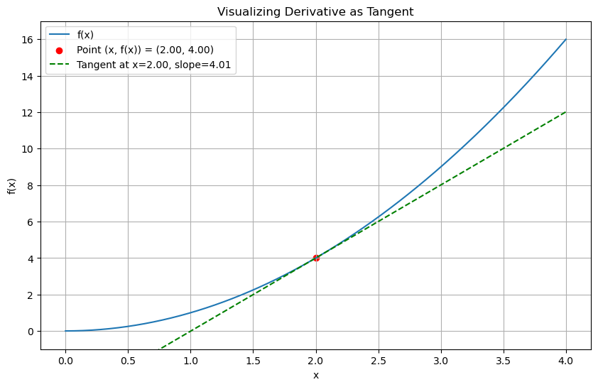
# Function to plot and show derivative as tangent
def visualize_derivative(func, x, h=0.01):
    y = func(x)
    slope = (func(x + h) - func(x)) / h
    tangent = lambda t: slope * (t - x) + y

    x_vals = np.linspace(x - 2, x + 2, 400)
    y_vals = func(x_vals)
    tangent_vals = tangent(x_vals)

    plt.figure(figsize=(10, 6))
    plt.plot(x_vals, y_vals, label='f(x)')
    plt.scatter(x, y, color='red', label=f'Point (x, f(x)) = ({x:.2f}, {y:.2f})')
    plt.plot(x_vals, tangent_vals, '--g', label=f'Tangent at x={x:.2f}, slope={slope:.2f}')
    plt.xlabel('x')
    plt.ylabel('f(x)')
    plt.title('Visualizing Derivative as Tangent')
    plt.legend()
    plt.grid(True)
    plt.ylim(min(y_vals) - 1, max(y_vals) + 1)
    plt.show()

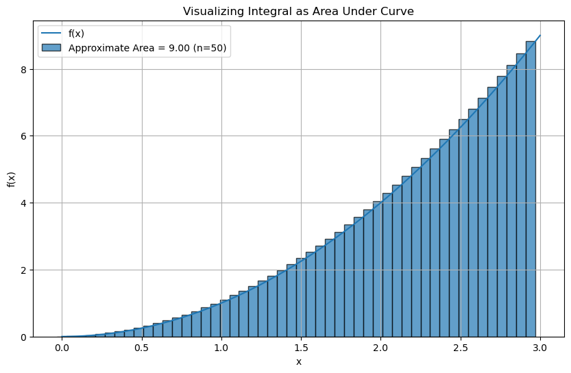
# Function to approximate integral using rectangles
def visualize_integral(func, a, b, n=50):
    x = np.linspace(a, b, n+1)
    dx = (b - a) / n
    x_mid = (x[:-1] + x[1:]) / 2
    y_mid = func(x_mid)
    area = np.sum(y_mid * dx)

    x_fine = np.linspace(a, b, 400)
    y_fine = func(x_fine)

    plt.figure(figsize=(10, 6))
    plt.plot(x_fine, y_fine, label='f(x)')
    plt.bar(x[:-1], y_mid, width=dx, alpha=0.7, edgecolor='black', label=f'Approximate Area = {area:.2f} (n={n})')
    plt.xlabel('x')
    plt.ylabel('f(x)')
    plt.title('Visualizing Integral as Area Under Curve')
    plt.legend()
    plt.grid(True)
    plt.show()

# Example function: f(x) = x^2
def f(x):
    return x**2

# Visualize the derivative at x = 2
visualize_derivative(f, 2)

# Visualize the integral of f(x) from 0 to 3
visualize_integral(f, 0, 3)

_images/880bac75538e31073b12564019f538072547bfa6ff8c6523f82801ac7bc5b3f6.png

_images/749020443553ca85c78c3e4314f891bbe846bdb9e3c969b14ec77288faeeba69.png

# Your code here