Linear Model Family#
Meet the Family: Simple, Multiple & Generalized Regression
“Every family has that one member who thinks they can explain everything with a straight line.” — Anonymous Data Scientist 😅
Welcome to the Linear Model Family, where:
Everyone loves straight lines,
Each cousin adds more variables,
And the distant uncle GLM shows up talking about log-odds at dinner.
👪 Meet the Family#
Let’s meet the key members of the Linear Model clan — one equation at a time.
🧍 Simple Linear Regression#
(The minimalist sibling)
[ \hat{y} = \beta_0 + \beta_1x ]
One input feature (
x)One output (
y)One slope, one intercept — simple and dramatic.
📊 Example: Predict sales from ad spend.
“Every extra dollar in advertising brings an extra $0.10 in sales.”
That’s it. Straightforward. No drama. Until marketing adds more variables…
👯♀️ Multiple Linear Regression#
(The overachiever sibling)
[ \hat{y} = \beta_0 + \beta_1x_1 + \beta_2x_2 + … + \beta_nx_n ]
When one variable isn’t enough, multiple regression joins the chat. Now we can model complex situations like:
📊 Example:
Predict sales using TV, radio, and social media ad spend.
Feature |
Coefficient |
Meaning |
|---|---|---|
TV Spend |
0.04 |
+\(0.04 in sales per \)1 spent |
Radio Spend |
0.08 |
+\(0.08 in sales per \)1 spent |
Social Spend |
0.01 |
“We’re trying…” |
🎯 Business Translation: “TV ads sell, radio works, and social media gives us likes but not customers.”
🧙 Generalized Linear Models (GLM)#
(The mysterious uncle with equations and wine)
When your dependent variable isn’t continuous (like 0/1, counts, or categories), you need a model that can flex — enter GLM.
GLM extends the linear model by adding:
A link function (to transform predictions)
A distribution for the target variable
Examples include:
Logistic Regression (for binary outcomes)
Poisson Regression (for count data)
Gamma Regression (for skewed continuous data)
📊 Example:
Predict whether a customer will buy (
1) or not (0) based on ad exposure.
GLM says: [ \text{logit}(p) = \beta_0 + \beta_1x_1 + \beta_2x_2 ]
Or in business English:
“Let’s use math to convert a yes/no question into something linear enough to make our computer happy.”
🧠 Concept Map#
Model Type |
Equation |
Target Type |
Business Example |
|---|---|---|---|
Simple Linear |
( y = \beta_0 + \beta_1x ) |
Continuous |
Predict sales from one ad channel |
Multiple Linear |
( y = \beta_0 + \sum \beta_i x_i ) |
Continuous |
Predict revenue from multiple ad channels |
Logistic (GLM) |
( \text{logit}(p) = \beta_0 + \sum \beta_i x_i ) |
Binary |
Predict if customer churns |
Poisson (GLM) |
( \log(\lambda) = \beta_0 + \sum \beta_i x_i ) |
Count |
Predict number of calls to customer support |
🎓 Business Analogy#
Think of regression models as chefs:
Model |
Chef Personality |
Kitchen Style |
|---|---|---|
Simple Linear |
Makes perfect grilled cheese |
1 ingredient, 1 rule |
Multiple Linear |
Manages a buffet |
Handles many dishes (features) |
GLM |
Fusion chef |
Adjusts recipes (distributions) depending on the dish |
“The recipe may change, but the secret sauce — linear thinking — stays the same.” 👨🍳
🧪 Practice Corner: “Predict the Profit” 💰#
You’re analyzing the following dataset:
TV |
Radio |
Social |
Sales |
|---|---|---|---|
100 |
50 |
20 |
15 |
200 |
60 |
25 |
25 |
300 |
80 |
30 |
35 |
Try this in your notebook:
💬 Interpret it like a business pro: “For every \(1 spent on TV ads, sales increase by \)0.05 — but we might be overspending on radio.” 🎯
🧮 Math Snack: Correlation ≠ Causation#
Regression models capture relationships, not reasons. If ice cream sales correlate with shark attacks, it doesn’t mean sharks love dessert. 🦈🍦
Always mix regression with business logic — not blind trust.
🧭 Recap#
Concept |
Description |
|---|---|
Simple Regression |
One variable, one prediction |
Multiple Regression |
Many variables, one outcome |
GLM |
Regression for non-continuous targets |
Coefficients |
Measure effect of each variable |
Intercept |
The baseline prediction |
Assumptions |
Linearity, independence, normal errors |
💬 Final Thought#
“Linear models are like spreadsheets — simple, powerful, and everywhere. You just need to know which cells to fill.” 📊
🔜 Next Up#
👉 Head to Mean Squared Error — where we learn how to measure prediction pain and teach our models to feel regret mathematically. 🧠💔
“Because every good model needs to know how wrong it was — politely, of course.” 😅
Recall that a linear model has the form \begin{align*} y & = \theta_0 + \theta_1 \cdot x_1 + \theta_2 \cdot x_2 + … + \theta_d \cdot x_d \end{align*} where \(x \in \mathbb{R}^d\) is a vector of features and \(y\) is the target. The \(\theta_j\) are the parameters of the model.
Linear regression will find a straight line that will try to best fit the data provided. It does so by learning the slope of the line, and the bais term (y-intercept)
Given a table:
size of house(int sq. ft) (x) |
price in $1000(y) |
|---|---|
450 |
100 |
324 |
78 |
844 |
123 |
Our hypothesis (prediction) is: $\(h_\theta(x) = \theta_0 + \theta_1x\)\( Will give us an equation of line that will predict the price. The above equation is nothing but the equation of line. __When we say the machine learns, we are actually adjusting the parameters \)\theta_0\( and \)\theta_1\(__. So for a new x (size of house) we will insert the value of x in the above equation and produce a value \)\hat y$ (our prediction)
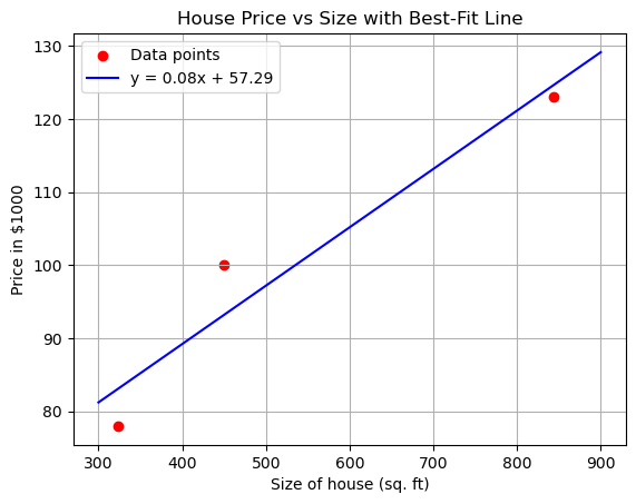
Below is a Python script that plots the equation \(y = mx + c\) using the provided data points and demonstrates how this equation relates to the linear model in the form of \(\theta\). The script first plots the data points and a best-fit line calculated using linear regression, then explains the connection between \(y = mx + c\) and the vectorized form \(h_\theta(x) = \theta^\top x\).
Explanation#
Plotting \(y = mx + c\): The script uses the data points provided (| Size of house (x) | Price (y) |) to compute the slope \(m\) (equivalent to \(\theta_1\)) and intercept \(c\) (equivalent to \(\theta_0\)) via linear regression. It then plots these points and the line \(y = mx + c\) using Matplotlib.
Relation to \(\theta\):
The linear equation \(y = mx + c\) is a specific case of the linear model \(h_\theta(x) = \theta_0 + \theta_1 x\), where:
\(c = \theta_0\) (the y-intercept or bias term),
\(m = \theta_1\) (the slope or weight of the feature \(x\)).
By defining \(x_0 = 1\) as a constant feature, we can extend the input \(x\) to a vector \([1, x]\), and the parameters to a vector \(\theta = [\theta_0, \theta_1]\).
The model then becomes \(h_\theta(x) = \theta^\top x = \theta_0 \cdot 1 + \theta_1 \cdot x\), which is mathematically equivalent to \(y = mx + c\).
This vectorized form \(\theta^\top x\) is commonly used in machine learning to generalize the model to multiple features, e.g., \(h_\theta(x) = \theta_0 + \theta_1 x_1 + \cdots + \theta_d x_d\) for \(d\) features.
Computation: The script calculates \(\theta\) using the normal equation, ensuring the line minimizes the Mean Squared Error (MSE) for the given data. The resulting \(\theta_0\) and \(\theta_1\) are printed and used to plot the line.
This demonstrates both the plotting of \(y = mx + c\) and its representation in the \(\theta\)-based notation of linear regression.
import numpy as np
import matplotlib.pyplot as plt

# Data points from the table
x = np.array([450, 324, 844])  # Size of house in sq. ft
y = np.array([100, 78, 123])   # Price in $1000

# Construct the design matrix X with bias term (x_0 = 1)
X = np.vstack([np.ones(len(x)), x]).T  # Shape: (3, 2), where each row is [1, x_i]

# Compute optimal parameters theta using the normal equation: theta = (X^T X)^(-1) X^T y
XtX = np.dot(X.T, X)
XtX_inv = np.linalg.inv(XtX)
Xty = np.dot(X.T, y)
theta = np.dot(XtX_inv, Xty)
theta_0, theta_1 = theta  # theta_0 is the intercept (c), theta_1 is the slope (m)

# Print the parameters
print(f"Parameters in theta form: theta_0 (intercept) = {theta_0:.2f}, theta_1 (slope) = {theta_1:.2f}")
print(f"In y = mx + c form: c = {theta_0:.2f}, m = {theta_1:.2f}")
print("The model can be written as:")
print(f"  h_theta(x) = {theta_0:.2f} + {theta_1:.2f} * x")
print("Or in vectorized form: h_theta(x) = theta^T x, where theta = [theta_0, theta_1] and x = [1, x]")

# Generate points for the best-fit line
x_line = np.linspace(300, 900, 100)  # Range covering the data points
y_line = theta_0 + theta_1 * x_line  # y = mx + c using computed theta_0 and theta_1

# Plot the data points and the best-fit line
plt.scatter(x, y, color='red', label='Data points')
plt.plot(x_line, y_line, color='blue', label=f'y = {theta_1:.2f}x + {theta_0:.2f}')
plt.xlabel('Size of house (sq. ft)')
plt.ylabel('Price in $1000')
plt.title('House Price vs Size with Best-Fit Line')
plt.legend()
plt.grid(True)
plt.show()
Parameters in theta form: theta_0 (intercept) = 57.29, theta_1 (slope) = 0.08
In y = mx + c form: c = 57.29, m = 0.08
The model can be written as:
  h_theta(x) = 57.29 + 0.08 * x
Or in vectorized form: h_theta(x) = theta^T x, where theta = [theta_0, theta_1] and x = [1, x]
# Your code here