
Regularisation — Ridge, Lasso, and Elastic Net
Giving Your Model a Budget
Polynomial features let the model fit curves. Without a constraint, it will fit every curve — including noise. Regularisation adds a penalty on the size of the coefficients, forcing the model to earn each parameter it uses. The result: models that generalise instead of memorise.
Why Regularise?
Without regularisation, a degree-30 polynomial fit to 100 points will interpolate the training data almost perfectly — and produce wild oscillations on new data.
| Problem | Cause | Regularisation fix |
|---|---|---|
| Large, unstable coefficients | Model overfit to noise | Penalise |
| Many near-zero features in result | Multicollinearity | Ridge shrinks them stably |
| Want automatic feature selection | High-dimensional data | Lasso zeros unimportant features |
| Both stability and sparsity | Mixed signal/noise | Elastic Net blends L1 + L2 |
Mathematical Formulation
The standard MSE objective:
Ridge (L2 regularisation)
Setting the gradient to zero gives the Ridge Normal Equation:
where is the identity with the top-left (bias) entry set to 0 — the intercept is not regularised.
Lasso (L1 regularisation)
No closed form — the L1 term is not differentiable at zero. The standard solver is coordinate descent using the soft-threshold operator:
where is the partial residual correlation for feature .
Elastic Net
Blends Ridge stability with Lasso sparsity. Particularly useful when features are correlated — Lasso arbitrarily picks one from a correlated group, Elastic Net keeps both.
Coordinate Descent for Lasso
Because has a kink at zero, we use the subgradient. For Lasso the update per coordinate has the closed-form soft-threshold solution:
where is the partial residual. Weights in the band collapse exactly to zero — that is the source of sparsity.
For comparison, the Ridge coordinate update has the closed form:
which shrinks but never reaches zero.
Why Lasso Produces Sparsity — Constraint Geometry
Visualising L1, L2, and Elastic Net Constraints
%matplotlib inline
import numpy as np
import matplotlib.pyplot as plt

fig_scale = 1.6

def plot_loss_interpretation():
    line = np.linspace(-1.5, 1.5, 1001)
    xx, yy = np.meshgrid(line, line)

    l2          = xx**2 + yy**2
    l1          = np.abs(xx) + np.abs(yy)
    rho         = 0.7
    elastic_net = rho * l1 + (1 - rho) * l2

    plt.figure(figsize=(5 * fig_scale, 4 * fig_scale))
    ax = plt.gca()

    en_c = plt.contour(xx, yy, elastic_net, levels=[1], linewidths=2 * fig_scale, colors='darkorange')
    l2_c = plt.contour(xx, yy, l2,          levels=[1], linewidths=2 * fig_scale, colors='c')
    l1_c = plt.contour(xx, yy, l1,          levels=[1], linewidths=2 * fig_scale, colors='navy')
    ax.set_aspect('equal')
    ax.spines['left'].set_position('center')
    ax.spines['right'].set_color('none')
    ax.spines['bottom'].set_position('center')
    ax.spines['top'].set_color('none')

    plt.clabel(en_c, inline=1, fontsize=12 * fig_scale, fmt={1.0: 'Elastic Net'}, manual=[(-0.6, -0.6)])
    plt.clabel(l2_c, inline=1, fontsize=12 * fig_scale, fmt={1.0: 'L2 (Ridge)'},  manual=[(-0.5, -0.5)])
    plt.clabel(l1_c, inline=1, fontsize=12 * fig_scale, fmt={1.0: 'L1 (Lasso)'},  manual=[(-0.5, -0.5)])

    x1 = np.linspace(0.5, 1.5, 100)
    x2 = np.linspace(-1.0, 1.5, 100)
    X1, X2 = np.meshgrid(x1, x2)
    Y = np.sqrt(np.square(X1 / 2 - 0.7) + np.square(X2 / 4 - 0.28))
    cp = plt.contour(X1, X2, Y)
    plt.clabel(cp, inline=1, fontsize=3)

    ax.tick_params(axis='both', pad=0)
    ax.scatter(1,    0,    c='navy', s=50 * fig_scale, zorder=5, label='Lasso optimum (on axis = zero)')
    ax.scatter(0.89, 0.42, c='c',   s=50 * fig_scale, zorder=5, label='Ridge optimum (off axis)')
    ax.legend(loc='lower right', fontsize=9 * fig_scale)
    ax.set_title('Constraint geometry: L1 corners produce sparsity', fontsize=10 * fig_scale)

    plt.tight_layout()
    plt.show()

plot_loss_interpretation()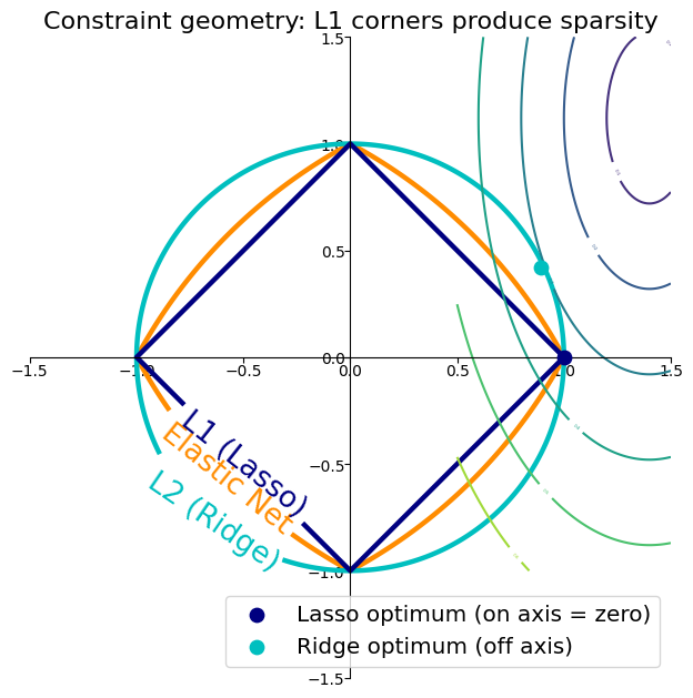
From-Scratch Implementations — OLS, Ridge, and Lasso
All three solvers operate on a degree-30 polynomial fit, demonstrating how regularisation tames wild overfitting.
%matplotlib inline
import numpy as np
from scipy.linalg import solve
import matplotlib.pyplot as plt

np.random.seed(42)
m = 100
X_raw = 6 * np.random.rand(m, 1) - 3
y_raw = 0.5 * X_raw**2 + X_raw + 2 + np.random.randn(m, 1)
X_new = np.linspace(-3, 3, 100).reshape(-1, 1)

degree = 30
def create_polynomial_features(X, degree):
    X_poly = np.ones((X.shape[0], 1))
    for d in range(1, degree + 1):
        X_poly = np.hstack((X_poly, X**d))
    return X_poly

X_poly     = create_polynomial_features(X_raw, degree)
X_new_poly = create_polynomial_features(X_new, degree)
mean_ = np.mean(X_poly[:, 1:], axis=0)
std_  = np.std(X_poly[:, 1:], axis=0); std_[std_ < 1e-8] = 1.0
X_ps     = X_poly.copy();     X_ps[:, 1:]     = (X_poly[:, 1:]     - mean_) / std_
X_new_ps = X_new_poly.copy(); X_new_ps[:, 1:] = (X_new_poly[:, 1:] - mean_) / std_

def linear_normal_equation(X, y):
    try:
        return solve(X.T @ X, X.T @ y, assume_a='pos')
    except Exception:
        return np.linalg.pinv(X.T @ X) @ (X.T @ y)

def linear_gradient_descent(X, y, learning_rate=0.01, n_iterations=1000):
    n_s, n_f = X.shape
    theta = np.zeros((n_f, 1))
    for _ in range(n_iterations):
        theta -= learning_rate * (1/n_s) * X.T @ (X @ theta - y)
    return theta

def ridge_normal_equation(X, y, lambda_reg):
    n_f = X.shape[1]
    I = np.eye(n_f); I[0, 0] = 0
    return solve(X.T @ X + lambda_reg * I, X.T @ y, assume_a='pos')

def ridge_gradient_descent(X, y, lambda_reg, learning_rate=0.01, n_iterations=1000):
    n_s, n_f = X.shape
    theta = np.zeros((n_f, 1))
    for _ in range(n_iterations):
        penalty = lambda_reg * np.vstack([0, theta[1:]])
        theta  -= learning_rate * ((1/n_s) * X.T @ (X @ theta - y) + penalty)
    return theta

def lasso_coordinate_descent(X, y, lambda_reg, max_iter=1000, tol=1e-4):
    n_s, n_f = X.shape
    theta = np.zeros((n_f, 1))
    y = y.reshape(-1, 1)
    for _ in range(max_iter):
        old = theta.copy()
        for j in range(n_f):
            Xj  = X[:, j:j+1]
            rho = (Xj * (y - X @ theta + Xj * theta[j])).sum() / n_s
            if j == 0:
                theta[j] = rho
            else:
                denom = float(Xj.T @ Xj) / n_s
                if   rho < -lambda_reg: theta[j] = (rho + lambda_reg) / denom
                elif rho >  lambda_reg: theta[j] = (rho - lambda_reg) / denom
                else:                   theta[j] = 0.0
        if np.linalg.norm(theta - old) < tol:
            break
    return theta

lam = 0.1
lr  = 0.005
iters = 2000
th_ols_ne  = linear_normal_equation(X_ps, y_raw)
th_ols_gd  = linear_gradient_descent(X_ps, y_raw, lr, iters)
th_ridge_ne = ridge_normal_equation(X_ps, y_raw, lam)
th_ridge_gd = ridge_gradient_descent(X_ps, y_raw, lam, lr, iters)
th_lasso    = lasso_coordinate_descent(X_ps, y_raw, lam)

fig, ax = plt.subplots(figsize=(12, 6))
ax.scatter(X_raw, y_raw, color='black', alpha=0.4, s=15, label='Data', zorder=3)
for th, color, ls, label in [
    (th_ols_ne,   'orange',    '-',  'OLS (Normal Eq)'),
    (th_ols_gd,   'black',     '--', 'OLS (Grad Desc)'),
    (th_ridge_ne, 'steelblue', '-',  f'Ridge NE (λ={lam})'),
    (th_ridge_gd, 'green',     '--', f'Ridge GD (λ={lam})'),
    (th_lasso,    'tomato',    '-',  f'Lasso CD (λ={lam})'),
]:
    ax.plot(X_new, np.clip(X_new_ps @ th, -5, 20), color=color, linestyle=ls, linewidth=1.8, label=label)
ax.set_ylim(-3, 18)
ax.legend(fontsize=9)
ax.set_title(f'Degree-{degree} polynomial: OLS vs Ridge vs Lasso')
ax.set_xlabel('x'); ax.set_ylabel('y')
plt.tight_layout(); plt.show()

nz = int(np.sum(np.abs(th_lasso) > 1e-6))
print(f'Lasso: {nz} non-zero coefficients out of {th_lasso.shape[0]}')
/var/folders/93/7lt42x5j7m39kz7wxbcghvrm0000gn/T/ipykernel_68029/2838958339.py:28: RuntimeWarning: divide by zero encountered in matmul
return solve(X.T @ X, X.T @ y, assume_a='pos')
/var/folders/93/7lt42x5j7m39kz7wxbcghvrm0000gn/T/ipykernel_68029/2838958339.py:28: RuntimeWarning: overflow encountered in matmul
return solve(X.T @ X, X.T @ y, assume_a='pos')
/var/folders/93/7lt42x5j7m39kz7wxbcghvrm0000gn/T/ipykernel_68029/2838958339.py:28: RuntimeWarning: invalid value encountered in matmul
return solve(X.T @ X, X.T @ y, assume_a='pos')
/var/folders/93/7lt42x5j7m39kz7wxbcghvrm0000gn/T/ipykernel_68029/2838958339.py:30: RuntimeWarning: divide by zero encountered in matmul
return np.linalg.pinv(X.T @ X) @ (X.T @ y)
/var/folders/93/7lt42x5j7m39kz7wxbcghvrm0000gn/T/ipykernel_68029/2838958339.py:30: RuntimeWarning: overflow encountered in matmul
return np.linalg.pinv(X.T @ X) @ (X.T @ y)
/var/folders/93/7lt42x5j7m39kz7wxbcghvrm0000gn/T/ipykernel_68029/2838958339.py:30: RuntimeWarning: invalid value encountered in matmul
return np.linalg.pinv(X.T @ X) @ (X.T @ y)
/Volumes/MacSSD/01_Projects/Chandravesh-ML-Research/projects/jupyter-books/.venv/lib/python3.10/site-packages/numpy/linalg/_linalg.py:3383: RuntimeWarning: divide by zero encountered in matmul
return _core_matmul(x1, x2)
/Volumes/MacSSD/01_Projects/Chandravesh-ML-Research/projects/jupyter-books/.venv/lib/python3.10/site-packages/numpy/linalg/_linalg.py:3383: RuntimeWarning: overflow encountered in matmul
return _core_matmul(x1, x2)
/Volumes/MacSSD/01_Projects/Chandravesh-ML-Research/projects/jupyter-books/.venv/lib/python3.10/site-packages/numpy/linalg/_linalg.py:3383: RuntimeWarning: invalid value encountered in matmul
return _core_matmul(x1, x2)
/var/folders/93/7lt42x5j7m39kz7wxbcghvrm0000gn/T/ipykernel_68029/2838958339.py:36: RuntimeWarning: divide by zero encountered in matmul
theta -= learning_rate * (1/n_s) * X.T @ (X @ theta - y)
/var/folders/93/7lt42x5j7m39kz7wxbcghvrm0000gn/T/ipykernel_68029/2838958339.py:36: RuntimeWarning: overflow encountered in matmul
theta -= learning_rate * (1/n_s) * X.T @ (X @ theta - y)
/var/folders/93/7lt42x5j7m39kz7wxbcghvrm0000gn/T/ipykernel_68029/2838958339.py:36: RuntimeWarning: invalid value encountered in matmul
theta -= learning_rate * (1/n_s) * X.T @ (X @ theta - y)
/var/folders/93/7lt42x5j7m39kz7wxbcghvrm0000gn/T/ipykernel_68029/2838958339.py:42: RuntimeWarning: divide by zero encountered in matmul
return solve(X.T @ X + lambda_reg * I, X.T @ y, assume_a='pos')
/var/folders/93/7lt42x5j7m39kz7wxbcghvrm0000gn/T/ipykernel_68029/2838958339.py:42: RuntimeWarning: overflow encountered in matmul
return solve(X.T @ X + lambda_reg * I, X.T @ y, assume_a='pos')
/var/folders/93/7lt42x5j7m39kz7wxbcghvrm0000gn/T/ipykernel_68029/2838958339.py:42: RuntimeWarning: invalid value encountered in matmul
return solve(X.T @ X + lambda_reg * I, X.T @ y, assume_a='pos')
/var/folders/93/7lt42x5j7m39kz7wxbcghvrm0000gn/T/ipykernel_68029/2838958339.py:49: RuntimeWarning: divide by zero encountered in matmul
theta -= learning_rate * ((1/n_s) * X.T @ (X @ theta - y) + penalty)
/var/folders/93/7lt42x5j7m39kz7wxbcghvrm0000gn/T/ipykernel_68029/2838958339.py:49: RuntimeWarning: overflow encountered in matmul
theta -= learning_rate * ((1/n_s) * X.T @ (X @ theta - y) + penalty)
/var/folders/93/7lt42x5j7m39kz7wxbcghvrm0000gn/T/ipykernel_68029/2838958339.py:49: RuntimeWarning: invalid value encountered in matmul
theta -= learning_rate * ((1/n_s) * X.T @ (X @ theta - y) + penalty)
/var/folders/93/7lt42x5j7m39kz7wxbcghvrm0000gn/T/ipykernel_68029/2838958339.py:60: RuntimeWarning: divide by zero encountered in matmul
rho = (Xj * (y - X @ theta + Xj * theta[j])).sum() / n_s
/var/folders/93/7lt42x5j7m39kz7wxbcghvrm0000gn/T/ipykernel_68029/2838958339.py:60: RuntimeWarning: overflow encountered in matmul
rho = (Xj * (y - X @ theta + Xj * theta[j])).sum() / n_s
/var/folders/93/7lt42x5j7m39kz7wxbcghvrm0000gn/T/ipykernel_68029/2838958339.py:60: RuntimeWarning: invalid value encountered in matmul
rho = (Xj * (y - X @ theta + Xj * theta[j])).sum() / n_s
/var/folders/93/7lt42x5j7m39kz7wxbcghvrm0000gn/T/ipykernel_68029/2838958339.py:64: DeprecationWarning: Conversion of an array with ndim > 0 to a scalar is deprecated, and will error in future. Ensure you extract a single element from your array before performing this operation. (Deprecated NumPy 1.25.)
denom = float(Xj.T @ Xj) / n_s
/var/folders/93/7lt42x5j7m39kz7wxbcghvrm0000gn/T/ipykernel_68029/2838958339.py:90: RuntimeWarning: divide by zero encountered in matmul
ax.plot(X_new, np.clip(X_new_ps @ th, -5, 20), color=color, linestyle=ls, linewidth=1.8, label=label)
/var/folders/93/7lt42x5j7m39kz7wxbcghvrm0000gn/T/ipykernel_68029/2838958339.py:90: RuntimeWarning: overflow encountered in matmul
ax.plot(X_new, np.clip(X_new_ps @ th, -5, 20), color=color, linestyle=ls, linewidth=1.8, label=label)
/var/folders/93/7lt42x5j7m39kz7wxbcghvrm0000gn/T/ipykernel_68029/2838958339.py:90: RuntimeWarning: invalid value encountered in matmul
ax.plot(X_new, np.clip(X_new_ps @ th, -5, 20), color=color, linestyle=ls, linewidth=1.8, label=label)
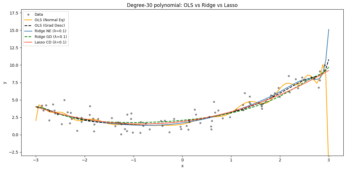
Lasso: 3 non-zero coefficients out of 31
Coefficient Paths — How Shrinks Parameters
As increases: Ridge shrinks smoothly, Lasso zeroes features one by one.
%matplotlib inline
import warnings
warnings.filterwarnings('ignore')
import numpy as np
import matplotlib.pyplot as plt
from sklearn.datasets import load_diabetes
from sklearn.linear_model import Ridge, lars_path

X_d, y_d = load_diabetes(return_X_y=True)

alphas = np.logspace(-5, 2, 60)
ridge_coefs = [Ridge(alpha=a, fit_intercept=False).fit(X_d, y_d).coef_ for a in alphas]

_, _, lasso_coefs = lars_path(X_d, y_d, method='lasso')
xx = np.sum(np.abs(lasso_coefs.T), axis=1)

fig, axes = plt.subplots(1, 2, figsize=(14, 5))

axes[0].plot(alphas, ridge_coefs)
axes[0].set_xscale('log')
axes[0].set_xlabel(r'Regularisation strength $\lambda$')
axes[0].set_ylabel('Coefficient magnitude')
axes[0].set_title(r'Ridge: all coefficients shrink smoothly toward 0')
axes[0].axis('tight')

axes[1].plot(3500 - xx, lasso_coefs.T)
axes[1].set_xlabel(r'Regularisation strength $\lambda$')
axes[1].set_ylabel('Coefficient magnitude')
axes[1].set_title('Lasso: coefficients hit zero and stay there (sparsity)')
axes[1].axis('tight')

plt.suptitle('Coefficient paths — Ridge vs Lasso on the diabetes dataset', y=1.01)
plt.tight_layout()
plt.show()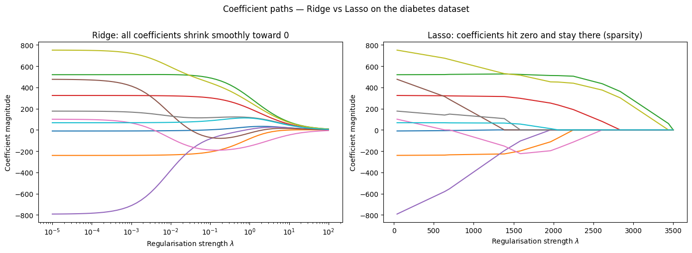
Ridge, Lasso, and Elastic Net with scikit-learn
%matplotlib inline
import numpy as np
import matplotlib.pyplot as plt
from sklearn.linear_model import Ridge, Lasso, ElasticNet
from sklearn.preprocessing import PolynomialFeatures, StandardScaler
from sklearn.pipeline import make_pipeline

np.random.seed(42)
m = 100
X = 6 * np.random.rand(m, 1) - 3
y = (0.5 * X**2 + X + 2 + np.random.randn(m, 1)).ravel()
X_new = np.linspace(-3, 3, 200).reshape(-1, 1)

degree = 15
configs = [
    ('OLS (no reg)',    make_pipeline(PolynomialFeatures(degree), StandardScaler(), Ridge(alpha=0)),      'grey',      '--'),
    ('Ridge α=1',      make_pipeline(PolynomialFeatures(degree), StandardScaler(), Ridge(alpha=1)),      'steelblue', '-'),
    ('Ridge α=10',     make_pipeline(PolynomialFeatures(degree), StandardScaler(), Ridge(alpha=10)),     'blue',      '-'),
    ('Lasso α=0.1',    make_pipeline(PolynomialFeatures(degree), StandardScaler(), Lasso(alpha=0.1, max_iter=10000)),   'tomato', '-'),
    ('ElasticNet',     make_pipeline(PolynomialFeatures(degree), StandardScaler(), ElasticNet(alpha=0.5, l1_ratio=0.5, max_iter=10000)), 'purple', '-'),
]

fig, ax = plt.subplots(figsize=(11, 5))
ax.scatter(X, y, color='black', alpha=0.3, s=15, label='Data', zorder=3)
for label, pipe, color, ls in configs:
    pipe.fit(X, y)
    ax.plot(X_new, np.clip(pipe.predict(X_new), -5, 20), color=color, linewidth=2, linestyle=ls, label=label)

ax.set_ylim(-3, 18)
ax.legend(fontsize=9)
ax.set_title(f'Degree-{degree} polynomial with different regularisers')
ax.set_xlabel('x'); ax.set_ylabel('y')
plt.tight_layout(); plt.show()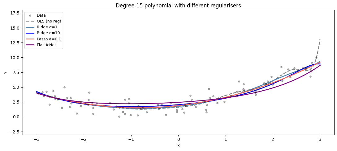
Choosing with Cross-Validation
%matplotlib inline
import numpy as np
import matplotlib.pyplot as plt
from sklearn.linear_model import Ridge, Lasso
from sklearn.datasets import make_regression
from sklearn.model_selection import cross_val_score
from sklearn.preprocessing import StandardScaler

X_cv, y_cv = make_regression(n_samples=50, n_features=100,
                             n_informative=5, noise=20, random_state=42)
scaler = StandardScaler()
X_cv_s = scaler.fit_transform(X_cv)

alphas = np.logspace(-2, 4, 100)
ridge_mse, lasso_mse = [], []

for alpha in alphas:
    ridge_mse.append(np.mean(-cross_val_score(
        Ridge(alpha=alpha, max_iter=10000), X_cv_s, y_cv,
        cv=5, scoring='neg_mean_squared_error')))
    lasso_mse.append(np.mean(-cross_val_score(
        Lasso(alpha=alpha, max_iter=10000), X_cv_s, y_cv,
        cv=5, scoring='neg_mean_squared_error')))

best_ridge = alphas[np.argmin(ridge_mse)]
best_lasso = alphas[np.argmin(lasso_mse)]

fig, ax = plt.subplots(figsize=(10, 5))
ax.semilogx(alphas, ridge_mse, color='steelblue', linewidth=2, label='Ridge')
ax.semilogx(alphas, lasso_mse, color='tomato',    linewidth=2, label='Lasso')
ax.scatter(best_ridge, min(ridge_mse), color='steelblue', s=100, zorder=5,
           label=f'Best Ridge (alpha={best_ridge:.1f})')
ax.scatter(best_lasso, min(lasso_mse), color='tomato',    s=100, zorder=5,
           label=f'Best Lasso (alpha={best_lasso:.1f})')
ax.axhline(min(ridge_mse), color='steelblue', linestyle=':', alpha=0.4)
ax.axhline(min(lasso_mse), color='tomato',    linestyle=':', alpha=0.4)
ax.set_xlabel(r'Regularisation strength $\alpha$')
ax.set_ylabel('5-fold CV MSE')
ax.set_title('Cross-validation alpha search\n(50 samples, 100 features, 5 informative)')
ax.legend(); ax.grid(True, which='both', alpha=0.3)
plt.tight_layout(); plt.show()

print(f"OLS (alpha~0) CV MSE : {ridge_mse[0]:.1f}")
print(f"Best Ridge CV MSE    : {min(ridge_mse):.1f}  (improvement: {100*(ridge_mse[0]-min(ridge_mse))/ridge_mse[0]:.1f}%)")
print(f"Best Lasso CV MSE    : {min(lasso_mse):.1f}  (improvement: {100*(lasso_mse[0]-min(lasso_mse))/lasso_mse[0]:.1f}%)")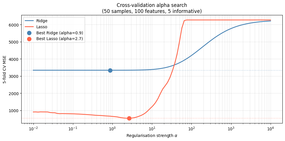
OLS (alpha~0) CV MSE : 3338.7
Best Ridge CV MSE    : 3338.2  (improvement: 0.0%)
Best Lasso CV MSE    : 539.3  (improvement: 40.4%)
Try It in the Browser
Ridge vs Lasso vs Elastic Net — Quick Reference
| Property | Ridge (L2) | Lasso (L1) | Elastic Net |
|---|---|---|---|
| Penalty | $\lambda\sum | \theta_j | |
| Closed-form? | Yes (modified Normal Eq) | No (coordinate descent) | No |
| Produces exact zeros? | No — shrinks only | Yes | Yes — fewer than Lasso |
| Handles correlated features? | Yes — distributes weight | No — picks one | Yes — groups correlated |
| Best when | Many small effects, multicollinearity | Sparse true signal | Correlated features + sparsity |
| sklearn class | Ridge / RidgeCV | Lasso / LassoCV | ElasticNet / ElasticNetCV |
Guided Practice
What is the main purpose of regularisation?
Which statement best distinguishes Lasso from Ridge?
What happens to Ridge coefficients as lambda increases toward infinity?
You have 50 samples and 200 features with only 8 truly predictive. Which regulariser is most appropriate?
%matplotlib inline
import numpy as np, matplotlib.pyplot as plt
from sklearn.preprocessing import PolynomialFeatures, StandardScaler

rng = np.random.default_rng(0)
n = 80
X_e = rng.uniform(-3, 3, (n, 1))
y_e = (0.5*X_e.ravel()**2 + X_e.ravel() + 2 + rng.normal(0, 1, n)).reshape(-1, 1)

pf = PolynomialFeatures(10, include_bias=True)
Xp = pf.fit_transform(X_e)
sc = StandardScaler(with_mean=False); Xp = sc.fit_transform(Xp)

# TODO: implement Ridge gradient descent
# gradient = (2/n)*X^T(X@theta - y) + 2*lambda*theta  (skip bias at index 0)
# Run 2000 steps with lr=0.01, lambda=0.5
# Plot fitted curve vs data
Hint
theta = np.zeros((Xp.shape[1], 1))
lam, lr = 0.5, 0.01
for _ in range(2000):
    res   = Xp @ theta - y_e
    pen   = np.vstack([0, theta[1:]])   # skip bias
    theta -= lr * ((2/n) * Xp.T @ res + 2*lam * pen)
Exercise 2 — Lasso feature selection
Generate 100 samples with 50 features where only 3 are truly predictive. Fit LassoCV and confirm it recovers those features.
import numpy as np
from sklearn.linear_model import LassoCV, Ridge
from sklearn.preprocessing import StandardScaler

rng = np.random.default_rng(7)
n, p = 100, 50
X2 = rng.normal(0, 1, (n, p))
true_coef = np.zeros(p)
true_coef[[3, 17, 42]] = [2.5, -1.8, 3.1]   # only 3 features matter
y2 = X2 @ true_coef + rng.normal(0, 1, n)

X2s = StandardScaler().fit_transform(X2)

# TODO: fit LassoCV, print which features have non-zero coefficients
# TODO: compare with Ridge — does Ridge zero out the noise features?
Exercise 3 — Elastic Net vs LassoCV vs RidgeCV comparison
from sklearn.linear_model import LassoCV, RidgeCV, ElasticNetCV
import numpy as np

# Use X2s and y2 from Exercise 2
# TODO: fit LassoCV, RidgeCV, ElasticNetCV
# Print best alpha and 5-fold CV MSE for each
Common Pitfalls
Summary
Key takeaways
| Concept | One-line meaning |
|---|---|
| Regularisation | Add a penalty on to force the model to earn each parameter |
| Ridge (L2) | Penalty — shrinks all coefficients smoothly, never to zero |
| Lasso (L1) | Penalty $\lambda\sum |
| Elastic Net | Blend of L1 + L2 — handles correlated features and gives sparsity |
| Why Lasso zeros | L1 ball has corners on axes — MSE ellipse touches corners more often than smooth L2 circle |
| Coordinate descent | Soft-threshold update per coordinate is the standard Lasso solver |
| Choosing | Cross-validation — RidgeCV / LassoCV automate this |
| Scale first | Always standardise features before regularising |
Next Up — Bias-Variance Tradeoff

You can now control overfitting. Next: understand the fundamental tension behind it.
The next notebook — Bias-Variance Tradeoff — gives the mathematical decomposition of generalisation error into bias (systematic error from underfitting) and variance (sensitivity to noise). It explains why regularisation helps, why you can never reduce both to zero, and how to diagnose which dominates your model.
Dependencies you already have: MSE definition, overfitting vs underfitting intuition, and the effect of $\lambda$ on coefficient magnitudes.