Non-Linear & Polynomial Features¶

Making Linear Models Curvy¶

OLS finds the best straight line. But real business data rarely behaves linearly. Polynomial features let you fit curves using the same linear algebra you already know: add $x^2$, $x^3$, interaction terms as new columns, then apply OLS as usual.

Why Go Beyond Linear?¶

Business scenario	Why it curves
Ad spend vs revenue	Diminishing returns — first dollars convert, last ones do not
Price vs demand	Steep drop at first, then flattens
Employee count vs output	Efficiency peaks, then overhead grows
Product age vs defect rate	Bathtub curve — high early, low mid-life, high again at end

What Is a Polynomial Feature?¶

A polynomial of degree $d$ in one variable:

\hat{y} = \theta_0 + \theta_1 x + \theta_2 x^2 + \cdots + \theta_d x^d

(1)

This is still linear in the parameters $\boldsymbol{\theta}$ . We rewrite it as $\hat{y} = \boldsymbol{\theta}^\top \mathbf{x}_{\text{poly}}$ where:

\mathbf{x}_{\text{poly}} = \begin{bmatrix}1 \\ x \\ x^2 \\ \vdots \\ x^d\end{bmatrix}

(2)

For two original features $x_1, x_2$ at degree 2, PolynomialFeatures expands to:

[1,\; x_1,\; x_2,\; x_1^2,\; x_1 x_2,\; x_2^2]

(3)

The interaction term $x_1 x_2$ captures joint effects — e.g. TV advertising combined with radio spend.

Polynomial terminology¶

A polynomial of degree $p$ is a function of the form:

a_p x^p + a_{p-1} x^{p-1} + \cdots + a_1 x + a_0

(4)

Visual Flow — Polynomial Pipeline¶

Scaling after polynomial expansion is essential — $x^{10}$ has a very different range than $x$ .

Polynomial Shape Gallery¶

%matplotlib inline
import numpy as np
import matplotlib.pyplot as plt
import warnings
warnings.filterwarnings('ignore')

x_vars = np.linspace(-2, 2, 200)

fig, axes = plt.subplots(1, 3, figsize=(14, 4))

axes[0].plot(x_vars, x_vars**2, color='steelblue', linewidth=2)
axes[0].set_title('Quadratic $x^2$')
axes[0].legend(['$x^2$'])

axes[1].plot(x_vars, x_vars**3, color='tomato', linewidth=2)
axes[1].set_title('Cubic $x^3$')
axes[1].legend(['$x^3$'])

axes[2].plot(x_vars, x_vars**3 + 2*x_vars**2 + x_vars + 1, color='green', linewidth=2)
axes[2].set_title('Mixed degree-3')
axes[2].legend(['$x^3 + 2x^2 + x + 1$'])

for ax in axes:
    ax.axhline(0, color='grey', linewidth=0.6, linestyle='--')
    ax.axvline(0, color='grey', linewidth=0.6, linestyle='--')

plt.suptitle('Polynomial shape gallery', y=1.02)
plt.tight_layout()
plt.show()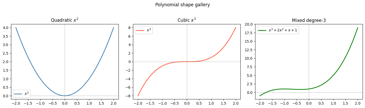

scikit-learn Pipeline: Fit Multiple Degrees¶

The canonical sklearn pattern: PolynomialFeatures → StandardScaler → LinearRegression.

%matplotlib inline
from sklearn.preprocessing import StandardScaler, PolynomialFeatures
from sklearn.pipeline import make_pipeline
from sklearn.linear_model import LinearRegression
import numpy as np
import matplotlib.pyplot as plt

np.random.seed(42)
m = 100
X = 6 * np.random.rand(m, 1) - 3
y = 0.5 * X**2 + X + 2 + np.random.randn(m, 1)

X_new = np.linspace(-3, 3, 200).reshape(-1, 1)

fig, ax = plt.subplots(figsize=(10, 5))
for style, width, degree in (("r-+", 2, 1), ("b--", 2, 2), ("g-", 1, 10), ("m-", 1, 20)):
    pipe = make_pipeline(
        PolynomialFeatures(degree=degree, include_bias=False),
        StandardScaler(),
        LinearRegression()
    )
    pipe.fit(X, y)
    label = f"{degree} degree{'s' if degree > 1 else ''}"
    ax.plot(X_new, pipe.predict(X_new), style, label=label, linewidth=width)

ax.plot(X, y, "k.", alpha=0.4, label="Training data")
ax.set_ylim(-2, 12)
ax.legend(loc="upper left")
ax.set_xlabel("$x$")
ax.set_ylabel("$y$")
ax.set_title("Polynomial regression — degree comparison")
plt.tight_layout()
plt.show()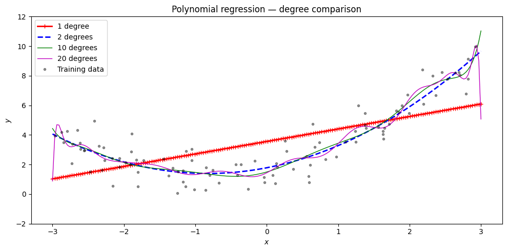

What you should see

Degree	Behaviour	Risk
1	Straight line — misses the curve	Underfitting
2	Follows the quadratic true shape	Good fit
10	Starts to wiggle at edges	Borderline overfitting
20	Wild oscillations at boundaries	Clear overfitting

Degree 2 is correct here because the true data-generating function is $0.5x^2 + x + 2$ .

Exploring the Expanded Feature Matrix¶

import numpy as np
from sklearn.preprocessing import PolynomialFeatures

# Single-feature expansion
X_sample = np.array([[2.0], [3.0]])
for degree in [1, 2, 3]:
    pf = PolynomialFeatures(degree=degree, include_bias=True)
    Xp = pf.fit_transform(X_sample)
    names = pf.get_feature_names_out(['x'])
    print(f"Degree {degree}: features={list(names)}")
    print(f"  Row 0 values: {Xp[0]}")

print()
# Two-feature expansion — shows interaction term
X2 = np.array([[2.0, 3.0]])
pf2 = PolynomialFeatures(degree=2, include_bias=True)
Xp2 = pf2.fit_transform(X2)
print("Two features, degree 2:")
print("  Features:", list(pf2.get_feature_names_out(['TV', 'Radio'])))
print("  Values:  ", Xp2[0])

Degree 1: features=['1', 'x']
  Row 0 values: [1. 2.]
Degree 2: features=['1', 'x', 'x^2']
  Row 0 values: [1. 2. 4.]
Degree 3: features=['1', 'x', 'x^2', 'x^3']
  Row 0 values: [1. 2. 4. 8.]

Two features, degree 2:
  Features: ['1', 'TV', 'Radio', 'TV^2', 'TV Radio', 'Radio^2']
  Values:   [1. 2. 3. 4. 6. 9.]

Intuition: Feature Space Expansion¶

Think of polynomial feature generation as bending the feature space:

Original 2D space: data points in $x$ vs $y$ — the relationship is curved.
Transformation: create $x^2$ as a new feature. Each point $(x_i, y_i)$ now lives in a 3D space $(x, x^2, y)$ .
Fit in the new space: in 3D, a flat plane fits the data well — linear regression works.
Map back: the flat plane in $(x, x^2, y)$ space becomes a parabola in the original $(x, y)$ space.

The model stays linear in $\boldsymbol{\theta}$ , but its decision surface in the original space is non-linear.

Under the Hood — Polynomial Regression from Scratch¶

The functions below implement polynomial feature generation and fitting via gradient descent without sklearn.

%matplotlib inline
import numpy as np
import matplotlib.pyplot as plt

def generate_polynomial_features(X, degree):
    """Return matrix where column i is X^(i+1), for i in 0..degree-1."""
    n_samples = X.shape[0]
    poly_features = np.empty((n_samples, degree))
    for i in range(1, degree + 1):
        poly_features[:, i - 1] = X ** i
    return poly_features

def fit_polynomial_regression(X_poly, y, learning_rate=0.01, n_iterations=1000):
    """Fit polynomial regression via gradient descent; returns coefficient vector."""
    n_samples, n_features = X_poly.shape
    coefficients = np.random.randn(n_features)
    X_poly = np.concatenate((np.ones((n_samples, 1)), X_poly), axis=1)
    coefficients = np.concatenate(([0], coefficients))
    for _ in range(n_iterations):
        y_predicted = np.dot(X_poly, coefficients)
        error = y_predicted - y
        gradients = (1 / n_samples) * np.dot(X_poly.T, error)
        coefficients -= learning_rate * gradients
    return coefficients

def predict_polynomial(X, coefficients):
    degree = len(coefficients) - 1
    X_poly = generate_polynomial_features(X, degree)
    X_poly = np.concatenate((np.ones((X.shape[0], 1)), X_poly), axis=1)
    return np.dot(X_poly, coefficients)

np.random.seed(42)
n_samples = 30
X_train = np.sort(np.random.rand(n_samples))
true_fn  = lambda x: np.cos(1.5 * np.pi * x)
y_train  = true_fn(X_train) + np.random.normal(0, 0.1, n_samples)

degrees = [3, 7, 15]
X_test  = np.linspace(0, 1, 100)

fig, axes = plt.subplots(1, 3, figsize=(14, 4))
for ax, degree in zip(axes, degrees):
    X_poly = generate_polynomial_features(X_train, degree)
    coef   = fit_polynomial_regression(X_poly, y_train, learning_rate=0.1, n_iterations=5000)
    y_pred = predict_polynomial(X_test, coef)
    ax.plot(X_test, true_fn(X_test), 'k-', label='True function')
    ax.plot(X_test, y_pred, 'r-', label=f'Degree {degree}')
    ax.scatter(X_train, y_train, edgecolor='b', s=20, label='Samples')
    ax.set_xlim(0, 1); ax.set_ylim(-2, 2)
    ax.legend(loc='best'); ax.set_title(f'Degree {degree}')

plt.suptitle('Polynomial regression from scratch (GD)', y=1.02)
plt.tight_layout()
plt.show()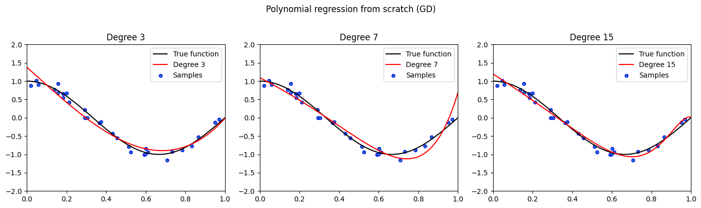

SVD-Based Polynomial Regression¶

For higher-degree polynomials, direct matrix inversion is numerically unstable. The PolynomialRegressionSVD class uses scipy.linalg.lstsq (SVD decomposition) for a more stable solution.

%matplotlib inline
import numpy as np
from scipy.linalg import lstsq
from sklearn.preprocessing import StandardScaler, PolynomialFeatures
import matplotlib.pyplot as plt

class PolynomialRegressionSVD:
    def __init__(self, degree=2):
        self.degree = degree
        self.poly   = PolynomialFeatures(degree=degree, include_bias=True)
        self.scaler = StandardScaler()

    def fit(self, X, y):
        X_poly = self.poly.fit_transform(X)
        if X_poly.shape[1] > 1:
            X_poly[:, 1:] = self.scaler.fit_transform(X_poly[:, 1:])
        self.coef_, _, _, _ = lstsq(X_poly, y)
        return self

    def predict(self, X):
        X_poly = self.poly.transform(X)
        if X_poly.shape[1] > 1:
            X_poly[:, 1:] = self.scaler.transform(X_poly[:, 1:])
        return X_poly @ self.coef_

np.random.seed(42)
X = 6 * np.random.rand(100, 1).astype(np.float64) - 3
y = (0.5 * X**2 + X + 2 + np.random.randn(100, 1)).astype(np.float64)
X_new = np.linspace(-3, 3, 200).reshape(-1, 1)

fig, ax = plt.subplots(figsize=(9, 5))
ax.plot(X, y, 'b.', alpha=0.4, label='Training data')
for degree, color in [(2, 'green'), (5, 'orange'), (10, 'tomato')]:
    model = PolynomialRegressionSVD(degree=degree)
    model.fit(X, y.ravel())
    ax.plot(X_new, model.predict(X_new), color=color, linewidth=2, label=f'SVD degree {degree}')
ax.set_ylim(-1, 14)
ax.legend()
ax.set_title('PolynomialRegressionSVD — numerically stable via lstsq')
plt.tight_layout()
plt.show()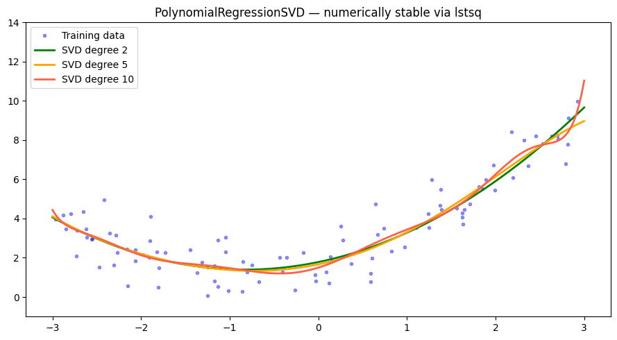

Gradient Descent Polynomial Regression¶

The PolynomialRegressionGD class fits polynomial regression via gradient descent with adaptive learning rate and convergence tolerance.

%matplotlib inline
import numpy as np
import matplotlib.pyplot as plt

class PolynomialRegressionGD:
    def __init__(self, degree, learning_rate=1e-3, n_iter=10000, tol=1e-4):
        self.degree        = degree
        self.learning_rate = learning_rate
        self.n_iter        = n_iter
        self.tol           = tol

    def _polynomial_features(self, X):
        features = [np.ones((X.shape[0], 1))]
        for d in range(1, self.degree + 1):
            features.append(X ** d)
        return np.hstack(features)

    def _standard_scale(self, X):
        self.mean_ = X.mean(axis=0)
        self.std_  = X.std(axis=0)
        self.std_[self.std_ < 1e-8] = 1.0
        return (X - self.mean_) / self.std_

    def fit(self, X, y):
        X_poly = self._polynomial_features(X)
        X_poly[:, 1:] = self._standard_scale(X_poly[:, 1:])
        m = X_poly.shape[0]
        self.theta = np.zeros((X_poly.shape[1], 1), dtype=np.float64)
        prev_loss  = np.inf
        for i in range(self.n_iter):
            y_pred = np.clip(X_poly @ self.theta, -1e100, 1e100)
            error  = y_pred - y
            loss   = float((error.T @ error) / m)
            if abs(prev_loss - loss) < self.tol:
                break
            prev_loss = loss
            grad      = (2 / m) * X_poly.T @ error
            effective_lr = self.learning_rate / (1 + 0.001 * i)
            self.theta  -= effective_lr * grad

    def predict(self, X):
        X_poly = self._polynomial_features(X)
        X_poly[:, 1:] = (X_poly[:, 1:] - self.mean_) / self.std_
        return np.clip(X_poly @ self.theta, -1e100, 1e100)

np.random.seed(42)
X = 6 * np.random.rand(100, 1).astype(np.float64) - 3
y = (0.5 * X**2 + X + 2 + np.random.randn(100, 1)).astype(np.float64)
X_new = np.linspace(-3, 3, 100).reshape(-1, 1).astype(np.float64)

fig, ax = plt.subplots(figsize=(10, 5))
for style, width, degree, lr in [
    ('r-+', 2, 1,  0.01),
    ('b--', 2, 2,  0.01),
    ('g-',  1, 3,  0.005),
    ('m-',  1, 10, 0.001),
]:
    model = PolynomialRegressionGD(degree=degree, learning_rate=lr, n_iter=20000)
    model.fit(X, y)
    ax.plot(X_new, model.predict(X_new), style, linewidth=width, label=f'Degree {degree}')

ax.plot(X, y, 'k.', alpha=0.3, label='Training data')
ax.set_ylim(-2, 14)
ax.legend()
ax.set_title('PolynomialRegressionGD — gradient descent, no sklearn')
plt.tight_layout()
plt.show()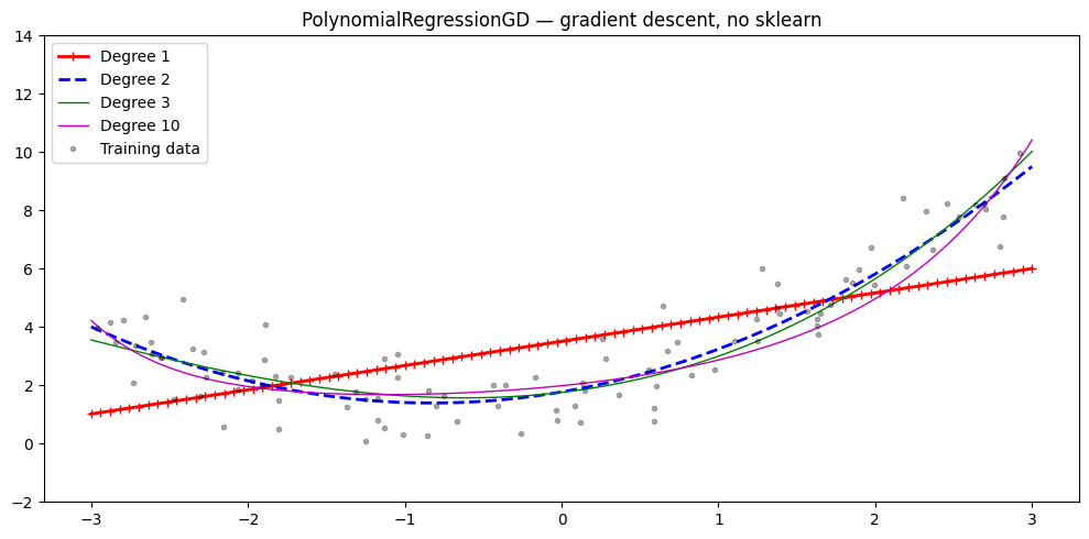

Overfitting vs Underfitting — The Degree Dial¶

Practical remedy for overfitting: add regularisation (Ridge / Lasso) — covered in the next notebook.

Try It in the Browser¶

Manually build a degree-2 polynomial design matrix and solve with the Normal Equations.

Guided Practice¶

Why do we add polynomial features to a regression model?¶

To capture curved relationships while keeping the model linear in its parametersCorrect. Polynomial terms expand the feature space; the model stays linear in theta, so OLS still applies.

To guarantee perfect generalisation on unseen dataNo feature transformation can guarantee perfect generalisation.

To convert the model into a classifier automaticallyPolynomial features remain within regression unless the task changes.

To remove the need for a bias termA bias term is still needed regardless of degree.

What is the main risk when the polynomial degree becomes very high?¶

The model always becomes simplerHigher-degree models are more flexible, not simpler.

Overfitting — the model fits noise instead of signalCorrect. Excessive flexibility can memorise training data and fail on new data.

OLS can no longer be usedOLS still applies regardless of degree — the design matrix just has more columns.

The model always predicts the training meanPredicting the mean is underfitting, not overfitting.

For two original features x1 and x2, how many terms does degree-2 PolynomialFeatures produce (including bias)?¶

4Close, but the interaction term x1*x2 adds one more. Count: 1 + 2 + 3 = 6.

6 — [1, x1, x2, x1^2, x1 x2, x2^2]Correct. Degree-2 expansion of 2 features gives 6 terms including the bias and the interaction.

5Five would miss one term. Count bias + 2 linear + 2 squared + 1 interaction = 6.

8Eight would be degree-3 expansion of 2 features.

Why must we scale features after polynomial expansion?¶

Because sklearn requires it by defaultScaling is a best practice, not a library constraint.

Because x^10 can be billions of times larger than x, causing numerical instabilityCorrect. Without scaling, higher-degree terms dominate and gradient descent or matrix inversion becomes unstable.

Because polynomial models cannot have negative predictionsPolynomial models can predict any real value regardless of scaling.

Because scaling removes the need for a bias termScaling and the bias term are independent concerns.

Exercises¶

Exercise 1 — Find the right degree¶

Generate data from a cubic function, then fit degrees 1–8. Plot training and validation MSE vs degree to find the sweet spot.

%matplotlib inline
import numpy as np
import matplotlib.pyplot as plt
from sklearn.preprocessing import PolynomialFeatures, StandardScaler
from sklearn.linear_model import LinearRegression
from sklearn.pipeline import make_pipeline
from sklearn.metrics import mean_squared_error

rng = np.random.default_rng(3)
n = 60
X_all = rng.uniform(-3, 3, (n, 1))
y_all = 0.3*X_all.ravel()**3 - X_all.ravel() + rng.normal(0, 1.5, n)

split = int(0.8 * n)
X_tr, X_val = X_all[:split], X_all[split:]
y_tr, y_val = y_all[:split], y_all[split:]

# TODO: for degrees 1..8, fit pipeline, compute train MSE and val MSE
# Plot both on one chart with degree on x-axis

train_errs, val_errs = [], []
for d in range(1, 9):
    pipe = make_pipeline(PolynomialFeatures(d), StandardScaler(), LinearRegression())
    pipe.fit(X_tr, y_tr)
    train_errs.append(mean_squared_error(y_tr, pipe.predict(X_tr)))
    val_errs.append(mean_squared_error(y_val, pipe.predict(X_val)))

Look for the degree where val MSE stops decreasing — that is your sweet spot.

Exercise 2 — Interaction terms for marketing¶

Generate synthetic marketing data where sales depend on an interaction between TV and Radio spend. Fit a degree-2 polynomial pipeline and confirm it recovers the interaction coefficient.

import numpy as np
from sklearn.preprocessing import PolynomialFeatures
from sklearn.linear_model import LinearRegression
from sklearn.pipeline import make_pipeline

rng = np.random.default_rng(7)
n = 200
TV    = rng.uniform(50, 250, n)
Radio = rng.uniform(10, 60, n)
X = np.column_stack([TV, Radio])
# True model: sales = 5 + 0.04*TV + 0.2*Radio + 0.003*TV*Radio + noise
y = 5 + 0.04*TV + 0.2*Radio + 0.003*TV*Radio + rng.normal(0, 2, n)

# TODO: fit degree-2 polynomial pipeline (no StandardScaler so coefficients are readable)
# Print feature names and corresponding coefficients

Exercise 3 — Compare all three implementations¶

On the same dataset ( $y = 0.5x^2 + x + 2$ , $n=100$ ), fit degree-2 polynomial regression using:

PolynomialRegressionSVD (from above)
PolynomialRegressionGD (from above)
sklearn make_pipeline(PolynomialFeatures(2), StandardScaler(), LinearRegression())

Print the MSE for each and confirm all three agree within a small tolerance.

# Your code here — use PolynomialRegressionSVD, PolynomialRegressionGD, and sklearn pipeline

Common Pitfalls¶

Summary¶

Concept	One-line meaning
Polynomial features	Add $x^2, x^3, \ldots$ and cross-terms as new columns to $\mathbf{X}$
Still linear in $\boldsymbol{\theta}$	OLS and gradient descent apply unchanged
Degree too low	Underfitting — model misses the curve
Degree too high	Overfitting — model fits noise, fails on new data
Scale after expanding	Essential for numerical stability
Interaction terms	$x_1 \cdot x_2$ captures joint feature effects
Feature count	Grows combinatorially with features and degree
Fix for overfitting	Regularisation (Ridge / Lasso) — next notebook

Next Up — Regularisation¶

Polynomial features let you fit curves. Regularisation keeps them from going wild.¶

The next notebook — Regularisation (Ridge & Lasso) — introduces a penalty term added to the loss that shrinks large coefficients. Ridge keeps all features but small, Lasso drives some to zero. Both are solved by a simple modification of the Normal Equations.

Dependencies you already have: the design matrix $\mathbf{X}$, coefficient interpretation, OLS, and the concept that high-degree polynomials overfit without constraint.