Ordinary Least Squares & the Normal Equations¶

The Closed-Form Shortcut to the Best-Fit Line¶

Gradient descent finds the minimum by walking downhill one step at a time. But for linear regression there is a one-shot algebraic solution that jumps directly to the bottom: the Normal Equations. This notebook derives it, implements it, and explains when to use it versus gradient descent.

From Gradient to Zero¶

In the gradients notebook we established the matrix gradient of the MSE loss:

\nabla_{\boldsymbol{\theta}}\, J = -\frac{1}{n}\mathbf{X}^\top\left(\mathbf{y} - \mathbf{X}\boldsymbol{\theta}\right)

(1)

Gradient descent keeps subtracting this until it is small. But what if we set it exactly to zero and solve?

-\frac{1}{n}\mathbf{X}^\top\left(\mathbf{y} - \mathbf{X}\boldsymbol{\theta}\right) = \mathbf{0}

(2)

\mathbf{X}^\top\mathbf{y} = \mathbf{X}^\top\mathbf{X}\,\boldsymbol{\theta}

(3)

If $\mathbf{X}^\top\mathbf{X}$ is invertible, multiply both sides by its inverse:

\boxed{\boldsymbol{\theta}^* = \left(\mathbf{X}^\top\mathbf{X}\right)^{-1}\mathbf{X}^\top\mathbf{y}}

(4)

This is the Normal Equation — the exact minimiser of MSE, computed in one step.

Visual: Two Paths to the Same Minimum¶

Matrix Dimensions Reference¶

For $n$ samples and $p$ features (plus a bias column):

Symbol	Meaning	Shape
$\mathbf{X}$	Design matrix (with bias column of 1s)	$(n,\; p+1)$
$\mathbf{y}$	Target vector	$(n,)$
$\mathbf{X}^\top\mathbf{X}$	Gram matrix	$(p+1,\; p+1)$
$(\mathbf{X}^\top\mathbf{X})^{-1}$	Inverse of Gram matrix	$(p+1,\; p+1)$
$\mathbf{X}^\top\mathbf{y}$	Moment vector	$(p+1,)$
$\boldsymbol{\theta}^*$	Optimal coefficients (incl. intercept)	$(p+1,)$

OLS from Scratch — NumPy Implementation¶

%matplotlib inline
import numpy as np
import matplotlib.pyplot as plt

# Toy advertising dataset
tv_spend = np.array([230, 44, 17, 151, 180, 8, 57, 120, 200, 100])
sales    = np.array([22, 10, 7, 18, 20, 3, 11, 15, 21, 13])

# Build design matrix X with bias column
n = len(tv_spend)
X = np.column_stack([np.ones(n), tv_spend])   # shape (n, 2)

# Normal Equations: theta* = (X^T X)^{-1} X^T y
theta = np.linalg.inv(X.T @ X) @ X.T @ sales
intercept, slope = theta

print(f"Intercept  (theta_0): {intercept:.4f}")
print(f"Slope      (theta_1): {slope:.4f}")
print(f"Interpretation: baseline sales = {intercept:.2f}; each $1 in TV adds {slope:.4f} in sales")

# Plot
x_line = np.linspace(0, 250, 200)
fig, ax = plt.subplots(figsize=(7, 4))
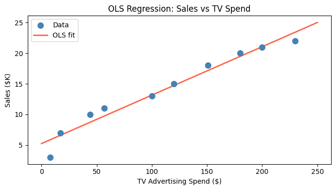
ax.scatter(tv_spend, sales, color='steelblue', s=70, zorder=3, label='Data')
ax.plot(x_line, intercept + slope * x_line, color='tomato', linewidth=2, label='OLS fit')
ax.set_xlabel('TV Advertising Spend ($)')
ax.set_ylabel('Sales ($K)')
ax.set_title('OLS Regression: Sales vs TV Spend')
ax.legend()
plt.tight_layout()
plt.show()

Intercept  (theta_0): 5.2428
Slope      (theta_1): 0.0791
Interpretation: baseline sales = 5.24; each $1 in TV adds 0.0791 in sales

OLS with scikit-learn¶

For production use, LinearRegression calls LAPACK’s least-squares solver internally.

%matplotlib inline
import numpy as np
import matplotlib.pyplot as plt
from sklearn.linear_model import LinearRegression
from sklearn.metrics import r2_score, mean_squared_error

rng = np.random.default_rng(42)
n = 80
X_feat = rng.uniform(0, 10, (n, 2))
true_coef = np.array([1.5, -0.8])
y = X_feat @ true_coef + 3.0 + rng.normal(0, 1.2, n)

model = LinearRegression().fit(X_feat, y)
y_hat = model.predict(X_feat)

print(f"Intercept: {model.intercept_:.4f}  (true: 3.0)")
print(f"Coef[0]:   {model.coef_[0]:.4f}   (true: 1.5)")
print(f"Coef[1]:   {model.coef_[1]:.4f}   (true: -0.8)")
print(f"R²:        {r2_score(y, y_hat):.4f}")
print(f"RMSE:      {np.sqrt(mean_squared_error(y, y_hat)):.4f}")

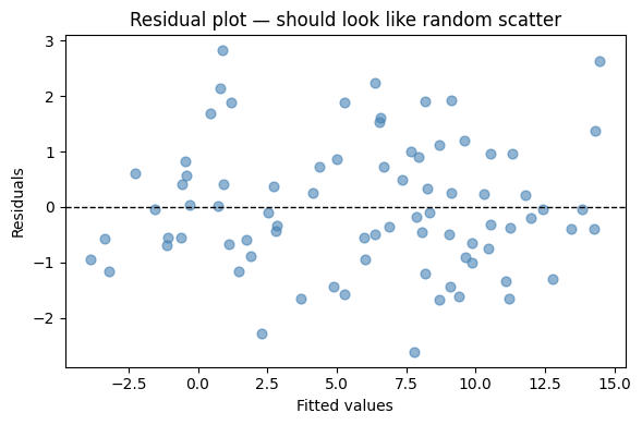
# Residual plot
fig, ax = plt.subplots(figsize=(6, 4))
ax.scatter(y_hat, y - y_hat, alpha=0.6, color='steelblue', s=40)
ax.axhline(0, color='black', linestyle='--', linewidth=1)
ax.set_xlabel('Fitted values')
ax.set_ylabel('Residuals')
ax.set_title('Residual plot — should look like random scatter')
plt.tight_layout()
plt.show()

Intercept: 2.9335  (true: 3.0)
Coef[0]:   1.5645   (true: 1.5)
Coef[1]:   -0.8477   (true: -0.8)
R²:        0.9458
RMSE:      1.1508

Full Diagnostic Summary with statsmodels¶

scikit-learn optimises for prediction. For inference — p-values, confidence intervals, VIF, autocorrelation tests — use statsmodels.

The cell below contains a reusable regression_summary_paragraph helper that formats the key diagnostics in plain language.

import pandas as pd
import statsmodels.api as sm
from statsmodels.stats.outliers_influence import variance_inflation_factor

def regression_summary_paragraph(model, 
                                alpha: float = 0.05,
                                vif_thresholds: tuple = (5, 10),
                                r2_thresholds: tuple = (0.3, 0.6)) -> str:
    """
    Creates a readable, multi-line summary from a fitted statsmodels OLS model.

    Returns a short, human-readable multi-line string (suitable for printing in
    notebooks or terminals). Keeps the same numeric checks as before but places
    results on separate lines for better readability.
    """
    n = int(model.nobs)
    r2 = model.rsquared
    adj_r2 = model.rsquared_adj
    fval = model.fvalue
    fp = model.f_pvalue

    # R² strength
    if r2 < r2_thresholds[0]:
        r2_qual = "weak"
    elif r2 < r2_thresholds[1]:
        r2_qual = "moderate"
    else:
        r2_qual = "strong"

    overall_sig = "statistically significant" if fp < alpha else "not statistically significant"

    # Coefficients (one line per predictor)
    coef_lines = []
    conf = model.conf_int(alpha).to_numpy()
    for var, coef, pval, ci_low, ci_high in zip(
        model.params.index,
        model.params,
        model.pvalues,
        conf[:, 0],
        conf[:, 1],
    ):
        if var == "const":
            continue
        sig_text = "significant" if pval < alpha else "not significant"
        coef_lines.append(
            f"{var}: {coef:+.3f} (p={pval:.4f}, 95% CI [{ci_low:.3f}, {ci_high:.3f}]) — {sig_text}"
        )

    # VIF (if applicable)
    vif_line = ""
    if model.df_model > 0:
        X = model.model.exog
        if X.shape[1] > 1:  # more than just intercept
            vif_df = pd.DataFrame({
                "variable": model.model.exog_names,
                "VIF": [variance_inflation_factor(X, i) for i in range(X.shape[1])],
            })
            vif_df = vif_df[vif_df["variable"] != "const"]
            vif_items = []
            for _, row in vif_df.iterrows():
                v = row["VIF"]
                if v < vif_thresholds[0]:
                    q = "low"
                elif v < vif_thresholds[1]:
                    q = "moderate"
                else:
                    q = "high"
                vif_items.append(f"{row['variable']} = {v:.2f} ({q})")
            if vif_items:
                vif_line = "VIFs: " + ", ".join(vif_items)

    # Durbin-Watson
    dw = sm.stats.durbin_watson(model.resid)
    dw_interp = (
        "approx 2 — no clear autocorrelation"
        if 1.5 <= dw <= 2.5
        else (f"{dw:.2f} — possible positive autocorrelation" if dw < 1.5 else f"{dw:.2f} — possible negative autocorrelation")
    )

    # Assemble multi-line output
    lines = []
    lines.append(f"Observations: {n}  |  R2 = {r2:.3f}  (adj R2 = {adj_r2:.3f})  --  {r2_qual}")
    lines.append(f"Overall model: {overall_sig}  |  F = {fval:.2f}, p = {fp:.4f}")
    lines.append("")
    lines.append("Coefficients:")
    if coef_lines:
        for cl in coef_lines:
            lines.append(f"  - {cl}")
    else:
        lines.append("  (no predictors besides intercept)")

    if vif_line:
        lines.append("")
        lines.append(vif_line)

    lines.append("")
    lines.append(f"Durbin-Watson: {dw_interp}")

    return "\n".join(lines)

# --- Minimal runnable example using synthetic data
import numpy as np
import pandas as pd

np.random.seed(0)
n = 200
# create a small advertising-style dataset (predictors only)
your_predictors_df = pd.DataFrame({
    "TV": np.random.normal(150, 30, size=n),
    "Radio": np.random.normal(30, 8, size=n),
    "Online": np.random.normal(50, 15, size=n),
})

# generate a target with known coefficients + noise
dependent_series = (
    10.0
    + 0.05 * your_predictors_df["TV"]
    + 0.4 * your_predictors_df["Radio"]
    - 0.02 * your_predictors_df["Online"]
    + np.random.normal(0, 3.0, size=n)
)
dependent_series = pd.Series(dependent_series, name="Sales")

# Fit OLS and show the human-readable paragraph
X = sm.add_constant(your_predictors_df)
model = sm.OLS(dependent_series, X).fit()

print("\nReadable summary:\n")
print(regression_summary_paragraph(model))


Readable summary:

Observations: 200  |  R2 = 0.551  (adj R2 = 0.544)  --  moderate
Overall model: statistically significant  |  F = 80.05, p = 0.0000

Coefficients:
  - TV: +0.048 (p=0.0000, 95% CI [0.035, 0.061]) — significant
  - Radio: +0.369 (p=0.0000, 95% CI [0.313, 0.424]) — significant
  - Online: -0.025 (p=0.0657, 95% CI [-0.052, 0.002]) — not significant

VIFs: TV = 1.01 (low), Radio = 1.04 (low), Online = 1.04 (low)

Durbin-Watson: approx 2 — no clear autocorrelation

Field	What it tells you
R²	Fraction of target variance explained (0–1; higher = better fit)
Adj R²	R² penalised for extra features — use for model comparison
F-stat / p	Is the model as a whole better than just predicting the mean?
Coef p-value	Is this predictor’s contribution distinguishable from noise?
95% CI	Range where the true coefficient lies with 95% confidence
VIF	Variance inflation factor: VIF > 10 signals severe multicollinearity
Durbin-Watson	Tests residual autocorrelation; ~2 is ideal, <1.5 or >2.5 is a red flag

In the example above, TV and Radio are significant, Online is not (p > 0.05). VIFs are all near 1, confirming no multicollinearity. Durbin-Watson near 2 means residuals are independent.

The Four OLS Assumptions¶

OLS gives the Best Linear Unbiased Estimator (BLUE) when these hold (Gauss-Markov theorem):

Violation	Consequence	Fix
Non-linearity	Biased coefficients	Add polynomial terms or transform features
Autocorrelated residuals	Underestimated standard errors	Use time-series models (ARIMA) or GLS
Heteroscedasticity	Wrong confidence intervals	Use robust standard errors or WLS
Multicollinearity (VIF > 10)	Unstable, inflated coefficients	Drop or combine collinear features; use Ridge
Outliers	Distorted fit	Investigate; use robust regression or winsorise

When to Use Normal Equations vs Gradient Descent¶

Try It in the Browser¶

Compute the Normal Equations solution from scratch using only Python built-ins.

Guided Practice¶

What is the main goal of Ordinary Least Squares?¶

To find coefficients that minimise the sum of squared residualsCorrect. OLS finds the exact parameter vector that minimises MSE in one step for linear models.

To maximise the number of features usedOLS does not select features — it fits all of them simultaneously.

To force all coefficients to zeroForcing coefficients to zero is regularisation (Lasso/Ridge), not OLS.

To maximise R-squared by adding featuresOLS minimises squared error; R² is a consequence, not the direct objective.

Why is the Normal Equation impractical for very large feature spaces (p >> 10 000)?¶

Because it requires a learning rateThe Normal Equation needs no learning rate — that is one of its advantages.

Because inverting a p x p matrix costs O(p³), which becomes prohibitiveCorrect. Matrix inversion scales cubically with the number of features, making it slow and memory-intensive at large scale.

Because it only works for binary targetsOLS is designed for continuous targets, not binary classification.

Because it cannot handle more than one featureThe Normal Equations extend naturally to any number of features via matrix operations.

A VIF of 14 for a predictor signals what problem?¶

The predictor is unimportantVIF measures collinearity with other predictors, not importance.

The residuals are autocorrelatedAutocorrelation is measured by the Durbin-Watson statistic, not VIF.

Severe multicollinearity — this predictor is strongly correlated with othersCorrect. VIF > 10 indicates the predictor shares so much variance with others that its coefficient estimate is unstable.

The model is overfittingOverfitting is assessed via train/test error gap, not VIF.

A Durbin-Watson statistic of 0.8 suggests what?¶

No multicollinearityDurbin-Watson tests autocorrelation, not multicollinearity.

Possible positive autocorrelation in the residualsCorrect. DW near 0 indicates strong positive autocorrelation; ideal is near 2; above 2.5 suggests negative autocorrelation.

Perfect model fitDW of 0.8 is actually a warning sign, not a sign of perfect fit.

HeteroscedasticityHeteroscedasticity is detected via a scale-location plot or Breusch-Pagan test, not DW.

Exercises¶

Exercise 1 — Normal Equations by hand¶

Given $n=4$ samples: $x=[1,2,3,4]$ , $y=[2,4,5,4]$ .

Build the design matrix $\mathbf{X}$ (add a column of ones).
Compute $\mathbf{X}^\top\mathbf{X}$ and $\mathbf{X}^\top\mathbf{y}$ .
Solve for $\boldsymbol{\theta}^*$ .
Compare with scikit-learn’s LinearRegression.

import numpy as np
from sklearn.linear_model import LinearRegression

x = np.array([1.0, 2.0, 3.0, 4.0])
y = np.array([2.0, 4.0, 5.0, 4.0])

# TODO: build X, compute Normal Equations solution, compare to sklearn

X = np.column_stack([np.ones(len(x)), x])
theta_ne = np.linalg.inv(X.T @ X) @ X.T @ y
print("Normal Equations:", theta_ne)

lr = LinearRegression().fit(x.reshape(-1,1), y)
print("sklearn intercept:", lr.intercept_, "slope:", lr.coef_[0])

Both should give intercept ≈ 1.5, slope ≈ 0.8.

Exercise 2 — Detect and interpret multicollinearity¶

Generate a dataset where two features are highly correlated (r > 0.95). Fit OLS, inspect the VIF values and coefficient confidence intervals. Describe what you observe.

import numpy as np
import pandas as pd
import statsmodels.api as sm
from statsmodels.stats.outliers_influence import variance_inflation_factor

rng = np.random.default_rng(5)
n = 100
x1 = rng.normal(0, 1, n)
x2 = x1 + rng.normal(0, 0.05, n)   # x2 almost identical to x1
y  = 2*x1 + 3 + rng.normal(0, 1, n)

df = pd.DataFrame({'x1': x1, 'x2': x2})
X  = sm.add_constant(df)

# TODO: fit OLS, print regression_summary_paragraph, observe VIF and CI width

Exercise 3 — OLS vs Gradient Descent speed comparison¶

Generate a dataset with $n=500$ rows and $p=50$ features. Time both approaches (Normal Equations via np.linalg.lstsq and your gradient descent implementation) and confirm they converge to the same $\boldsymbol{\theta}^*$ .

import numpy as np, time

rng = np.random.default_rng(99)
n, p = 500, 50
X_raw = rng.normal(0, 1, (n, p))
X = np.column_stack([np.ones(n), X_raw])
true_theta = rng.uniform(-2, 2, p+1)
y = X @ true_theta + rng.normal(0, 0.5, n)

# TODO: time Normal Equations solution
# TODO: time gradient descent (use the matrix form from gradients.ipynb)
# TODO: compare max absolute difference between the two theta vectors

/var/folders/93/7lt42x5j7m39kz7wxbcghvrm0000gn/T/ipykernel_67928/3962639806.py:8: RuntimeWarning: divide by zero encountered in matmul
  y = X @ true_theta + rng.normal(0, 0.5, n)
/var/folders/93/7lt42x5j7m39kz7wxbcghvrm0000gn/T/ipykernel_67928/3962639806.py:8: RuntimeWarning: overflow encountered in matmul
  y = X @ true_theta + rng.normal(0, 0.5, n)
/var/folders/93/7lt42x5j7m39kz7wxbcghvrm0000gn/T/ipykernel_67928/3962639806.py:8: RuntimeWarning: invalid value encountered in matmul
  y = X @ true_theta + rng.normal(0, 0.5, n)

Common Pitfalls¶

Summary¶

Concept	One-line meaning
Normal Equations	$\boldsymbol{\theta}^* = (\mathbf{X}^\top\mathbf{X})^{-1}\mathbf{X}^\top\mathbf{y}$ — exact MSE minimiser
Derivation	Set MSE gradient to zero; solve algebraically
Complexity	$O(p^3)$ for inversion — fast for small $p$ , slow for large $p$
vs GD	No iterations, no learning rate — but not scalable to huge feature spaces
R² / Adj R²	Variance explained; adj R² penalises extra features
VIF	Multicollinearity check; VIF > 10 = problem
Durbin-Watson	Autocorrelation check; ~2 = ideal
BLUE property	OLS gives the best linear unbiased estimator when all 4 assumptions hold

Next Up — Polynomial Features¶

OLS gives the best straight-line fit. But what if the relationship curves?¶

The next notebook — Polynomial Features — shows how to extend the linear model to capture non-linear patterns by adding $x^2$, $x^3$, and interaction terms as new features. The model stays linear in $\boldsymbol{\theta}$, so OLS still applies — but the decision boundary becomes a curve.

Dependencies you already have: the design matrix $\mathbf{X}$, coefficient interpretation, and the OLS solution formula. Polynomial features just expand $\mathbf{X}$ with new columns.