Gradients & Gradient Descent¶

How Machines Learn to Reduce Their Mistakes¶

You now know that minimising MSE is the goal. This notebook shows how that minimisation actually happens: by computing the gradient of the loss — the mathematical slope of the error surface — and taking a small step downhill at every iteration.

Why This Matters¶

In the MSE notebook we established the training objective:

J(\boldsymbol{\theta}) = \frac{1}{2n}\sum_{i=1}^{n}\left(y^{(i)} - \hat{y}^{(i)}\right)^2

(1)

We said “minimise this” — but how? For small problems the Normal Equations give a closed-form answer. For everything else (large datasets, neural networks, non-convex losses) we need gradient descent: an iterative algorithm that walks the loss surface downhill step by step.

What gradient descent powers	Examples
Linear & logistic regression training	scikit-learn `SGDClassifier`, `SGDRegressor`
All deep learning	PyTorch, TensorFlow, Keras
Large-scale recommendation systems	YouTube, Netflix ranking models
LLM pre-training	Every large language model ever trained

From Slope to Derivative¶

Slope of a straight line¶

For a straight line $f(x) = mx + b$ , the slope $m$ tells you: if I increase $x$ by 1, $f$ increases by $m$ .

Derivative of a curve¶

For a curved function the slope changes at every point. The derivative $\frac{df}{dx}$ gives the instantaneous slope at a specific $x$ :

\frac{df}{dx} = \lim_{h \to 0} \frac{f(x+h) - f(x)}{h}

(2)

For our purposes, three rules are enough:

Function	Derivative
$f(x) = c$ (constant)	0
$f(x) = x^n$	$n\,x^{n-1}$
$f(x) = (g(x))^2$	$2\,g(x)\cdot g'(x)$ (chain rule)

Partial derivative¶

When a function depends on multiple parameters — say $J(\theta_0, \theta_1)$ — a partial derivative $\frac{\partial J}{\partial \theta_j}$ treats all parameters except $\theta_j$ as constants and differentiates only with respect to $\theta_j$ .

\frac{\partial}{\partial \theta_j} J(\theta_0, \theta_1) = \text{slope of } J \text{ in the } \theta_j \text{ direction}

(3)

Deriving the Gradient of MSE¶

For simple linear regression, $\hat{y}^{(i)} = \theta_0 + \theta_1 x^{(i)}$ , the loss is:

J(\theta_0, \theta_1) = \frac{1}{2n}\sum_{i=1}^{n}\left(\color{#1f77b4}{y^{(i)}} - \color{#ff7f0e}{\theta_0 + \theta_1 x^{(i)}}\right)^2

(4)

Step 1 — let $e^{(i)} = y^{(i)} - \hat{y}^{(i)}$ (the residual).

J = \frac{1}{2n}\sum_i \left(e^{(i)}\right)^2

(5)

Step 2 — partial derivative with respect to $\theta_0$ (intercept).

Apply the chain rule: outer derivative of $u^2$ is $2u$ , inner derivative of $e^{(i)}$ with respect to $\theta_0$ is -1.

\frac{\partial J}{\partial \theta_0} = \frac{1}{2n}\sum_i 2\,e^{(i)}\cdot(-1) = -\frac{1}{n}\sum_i e^{(i)} = -\frac{1}{n}\sum_i\left(y^{(i)} - \hat{y}^{(i)}\right)

(6)

Step 3 — partial derivative with respect to $\theta_1$ (slope).

Inner derivative of $e^{(i)}$ with respect to $\theta_1$ is $-x^{(i)}$ .

\frac{\partial J}{\partial \theta_1} = -\frac{1}{n}\sum_i x^{(i)}\left(y^{(i)} - \hat{y}^{(i)}\right)

(7)

The gradient vector (one entry per parameter):

\nabla_{\boldsymbol{\theta}}\, J = \begin{bmatrix} \frac{\partial J}{\partial \theta_0} \\ \frac{\partial J}{\partial \theta_1} \end{bmatrix} = -\frac{1}{n}\begin{bmatrix} \sum_i\left(y^{(i)} - \hat{y}^{(i)}\right) \\ \sum_i x^{(i)}\left(y^{(i)} - \hat{y}^{(i)}\right) \end{bmatrix}

(8)

The gradient points uphill (toward greater loss). Taking a step in the negative gradient direction moves us downhill.

The Gradient Descent Update Rule¶

\boxed{\theta_j \;\leftarrow\; \theta_j \;-\; \alpha\,\frac{\partial J}{\partial \theta_j} \quad \text{for all } j \text{ simultaneously}}

(9)

where $\alpha > 0$ is the learning rate — the size of each step.

Repeat until convergence (loss stops decreasing meaningfully).

Visual Flow — One Gradient Descent Step¶

Each loop = one training epoch (batch GD) or one mini-batch step.

Worked Example — Gradient Descent from Scratch¶

%matplotlib inline
import numpy as np
import matplotlib.pyplot as plt

rng = np.random.default_rng(0)
x = np.array([1.0, 2, 3, 4, 5, 6])
y = 2.0 * x + 1.0 + rng.normal(0, 0.5, len(x))

# Gradient descent for y = t0 + t1*x
t0, t1 = 0.0, 0.0
lr = 0.02
n = len(x)
history = []

for step in range(200):
    y_hat = t0 + t1 * x
    residuals = y - y_hat
    loss = np.mean(residuals**2) / 2
    # Gradients (negative of what we derived, because residuals = y - y_hat)
    g0 = -residuals.mean()
    g1 = -(x * residuals).mean()
    t0 -= lr * g0
    t1 -= lr * g1
    history.append(loss)

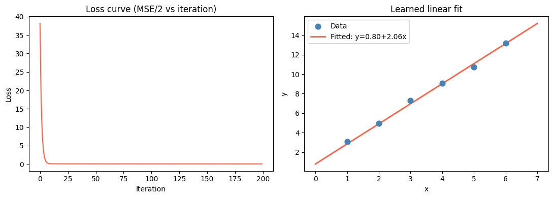
print(f"Learned: t0={t0:.4f}  t1={t1:.4f}  (true: t0=1.0  t1=2.0)")

fig, axes = plt.subplots(1, 2, figsize=(11, 4))

# Loss curve
axes[0].plot(history, color='tomato')
axes[0].set_title('Loss curve (MSE/2 vs iteration)')
axes[0].set_xlabel('Iteration')
axes[0].set_ylabel('Loss')

# Fit vs data
x_line = np.linspace(0, 7, 100)
axes[1].scatter(x, y, color='steelblue', s=60, label='Data', zorder=3)
axes[1].plot(x_line, t0 + t1 * x_line, color='tomato', linewidth=2, label=f'Fitted: y={t0:.2f}+{t1:.2f}x')
axes[1].set_title('Learned linear fit')
axes[1].set_xlabel('x')
axes[1].set_ylabel('y')
axes[1].legend()

plt.tight_layout()
plt.show()

Learned: t0=0.7969  t1=2.0569  (true: t0=1.0  t1=2.0)

Visualising the Loss Surface¶

%matplotlib inline
import numpy as np
import matplotlib.pyplot as plt

rng = np.random.default_rng(0)
x = np.array([1.0, 2, 3, 4, 5, 6])
y = 2.0 * x + 1.0 + rng.normal(0, 0.5, len(x))

# Grid over (t0, t1)
T0 = np.linspace(-2, 4, 120)
T1 = np.linspace(0, 4, 120)
Z = np.zeros((len(T0), len(T1)))
for i, a in enumerate(T0):
    for j, b in enumerate(T1):
        Z[i, j] = np.mean((y - (a + b * x))**2)

# Trace descent path
t0, t1 = -1.5, 0.2
path = [(t0, t1)]
lr = 0.02
for _ in range(60):
    res = y - (t0 + t1 * x)
    t0 -= lr * (-res.mean())
    t1 -= lr * (-(x * res).mean())
    path.append((t0, t1))

path = np.array(path)

fig, ax = plt.subplots(figsize=(7, 6))
cp = ax.contourf(T1, T0, Z, levels=40, cmap='RdYlGn_r')
plt.colorbar(cp, ax=ax, label='MSE loss')
ax.plot(path[:, 1], path[:, 0], 'w.-', linewidth=1.5, markersize=4, label='Descent path')
ax.plot(path[0, 1], path[0, 0], 'wo', markersize=8, label='Start')
ax.plot(path[-1, 1], path[-1, 0], 'w*', markersize=12, label='End')
ax.set_xlabel(r'$\theta_1$ (slope)')
ax.set_ylabel(r'$\theta_0$ (intercept)')
ax.set_title('Loss surface and gradient descent path')
ax.legend()
plt.tight_layout()
plt.show()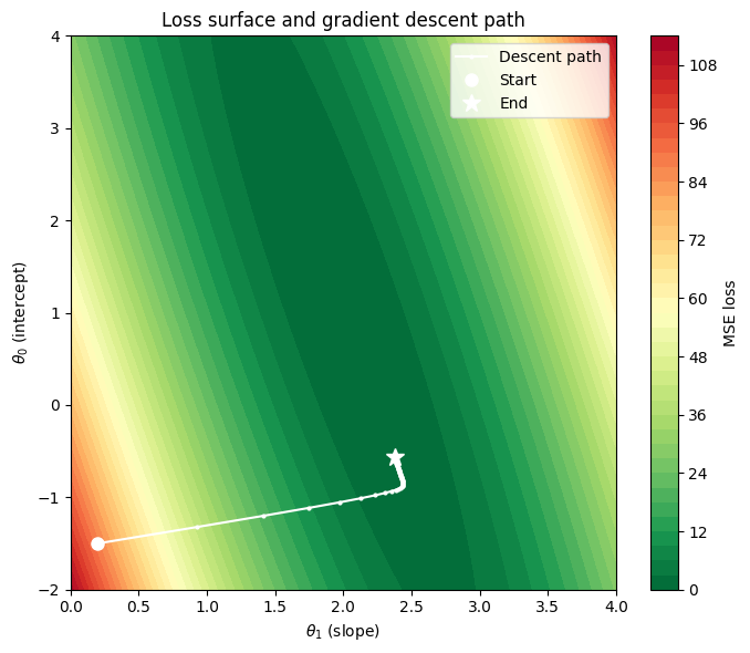

Learning Rate Sensitivity¶

%matplotlib inline
import numpy as np
import matplotlib.pyplot as plt

rng = np.random.default_rng(0)
x = np.array([1.0, 2, 3, 4, 5, 6])
y = 2.0 * x + 1.0 + rng.normal(0, 0.5, len(x))

def run_gd(lr, steps=80):
    t0, t1 = 0.0, 0.0
    losses = []
    for _ in range(steps):
        res = y - (t0 + t1 * x)
        loss = np.mean(res**2)
        losses.append(loss)
        t0 -= lr * (-res.mean())
        t1 -= lr * (-(x * res).mean())
    return losses

fig, ax = plt.subplots(figsize=(9, 4))
configs = [(0.001, 'Too small (lr=0.001)', 'steelblue'),
           (0.02,  'Good (lr=0.02)',        'green'),
           (0.25,  'Too large (lr=0.25)',   'tomato')]

for lr, label, color in configs:
    losses = run_gd(lr)
    # Clip for visibility
    clipped = np.clip(losses, 0, 20)
    ax.plot(clipped, color=color, label=label)

ax.set_xlabel('Iteration')
ax.set_ylabel('MSE loss (clipped at 20)')
ax.set_title('Effect of learning rate on convergence')
ax.legend()
plt.tight_layout()
plt.show()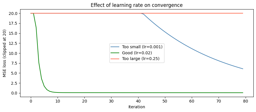

Learning rate behaviour summary

Learning rate	What happens	Loss curve shape
Too small	Slow convergence; many wasted iterations	Flat then very slowly decreasing
Good	Smooth convergence in reasonable steps	Steep drop then levels off
Too large	Overshoots; oscillates or diverges	Erratic or increasing

A practical starting point for gradient descent on normalised data is $\alpha = 0.01$ or 0.001. Always plot the loss curve.

Three Variants of Gradient Descent¶

In practice, mini-batch SGD dominates because it exploits GPU parallelism and adds enough noise to escape shallow local minima.

Try It in the Browser¶

Run one full gradient descent from scratch — edit the learning rate and see how convergence changes.

Matrix Form (Multiple Features)¶

For multiple features the model is $\hat{\mathbf{y}} = \mathbf{X}\boldsymbol{\theta}$ and the MSE gradient becomes a clean matrix expression:

\nabla_{\boldsymbol{\theta}}\, J = -\frac{1}{n}\mathbf{X}^\top\left(\mathbf{y} - \mathbf{X}\boldsymbol{\theta}\right)

(10)

The update rule is:

\boldsymbol{\theta} \;\leftarrow\; \boldsymbol{\theta} + \frac{\alpha}{n}\,\mathbf{X}^\top\left(\mathbf{y} - \mathbf{X}\boldsymbol{\theta}\right)

(11)

This is one matrix–vector multiply per iteration, making it efficient with NumPy or any BLAS library.

%matplotlib inline
import numpy as np

rng = np.random.default_rng(42)
n, d = 80, 3
X_raw = rng.normal(0, 1, (n, d))
true_theta = np.array([1.5, -0.8, 2.0])
y = X_raw @ true_theta + 0.5 + rng.normal(0, 0.3, n)

# Add bias column
X = np.column_stack([np.ones(n), X_raw])
theta = np.zeros(d + 1)
lr = 0.05
losses = []

for _ in range(300):
    y_hat = X @ theta
    residuals = y - y_hat
    losses.append(np.mean(residuals**2))
    theta += (lr / n) * X.T @ residuals

print("Learned theta:", np.round(theta, 4))
print("True [bias, t1, t2, t3]: [0.5, 1.5, -0.8, 2.0]")
print(f"Final MSE: {losses[-1]:.5f}")

Learned theta: [ 0.52    1.4798 -0.776   1.9671]
True [bias, t1, t2, t3]: [0.5, 1.5, -0.8, 2.0]
Final MSE: 0.09482

Guided Practice¶

What does the gradient of the loss tell you about a parameter?¶

The direction and rate at which the loss increases as that parameter increasesCorrect. The gradient points toward steeper loss increase; we move in the opposite direction to reduce loss.

The current value of the parameterThe gradient is a rate of change, not the parameter value itself.

How many training samples were usedSample count appears in the gradient formula as a denominator but is not what the gradient tells you.

The final optimal value of the parameterThe gradient only shows the local slope, not the global optimum.

If the gradient is close to zero, what might it indicate?¶

The learning rate is zeroA near-zero gradient is independent of the learning rate setting.

The model may be near a minimum, a plateau, or a saddle pointCorrect. Small gradients can mean convergence (good) or a flat region / saddle point (potentially bad for non-convex losses).

The dataset has too many featuresFeature count does not directly cause a near-zero gradient.

The model predicts the mean of yPredicting the mean would give zero gradient only for the intercept term, not all parameters.

Why do we subtract the gradient in the update rule rather than add it?¶

Because parameters must stay positiveParameters can be any real number; the sign convention is not about positivity.

Because the gradient points uphill; subtracting it moves us downhill toward lower lossCorrect. The gradient is the direction of steepest increase. To minimise, we move in the opposite direction.

Because adding would change the learning rateThe learning rate is a separate scalar multiplier; addition vs subtraction is about the direction of movement.

Because subtraction makes the update symmetricSymmetry is not the reason; the direction of optimisation is.

A model with a very large learning rate shows a loss that oscillates up and down. What is happening?¶

The training data has outliersOutliers affect loss magnitude but not the oscillating pattern caused by step-size issues.

The model has too many featuresFeature count is not the cause of oscillation from a large learning rate.

Each update overshoots the minimum, landing on the other side of the valleyCorrect. Large steps repeatedly jump past the minimum instead of converging to it.

The gradient is computed incorrectlyThe oscillation pattern here is due to step size, not a bug in the gradient formula.

Exercises¶

Exercise 1 — Manual one-step update¶

Given: $n=3$ samples, $x=[1,2,3]$ , $y=[3,5,7]$ , current $\theta_0=0$ , $\theta_1=0$ , $\alpha=0.1$ .

Compute $\hat{y}^{(i)}$ for each sample.
Compute the residuals $e^{(i)} = y^{(i)} - \hat{y}^{(i)}$ .
Compute $\frac{\partial J}{\partial \theta_0}$ and $\frac{\partial J}{\partial \theta_1}$ .
Compute the updated $\theta_0^{\text{new}}$ and $\theta_1^{\text{new}}$ .

import numpy as np

x = np.array([1.0, 2.0, 3.0])
y = np.array([3.0, 5.0, 7.0])
t0, t1 = 0.0, 0.0
lr = 0.1

# TODO: compute one gradient descent update step
# Expected result: t0 ~= 0.333, t1 ~= 0.733

y_hat     = t0 + t1 * x                        # [0, 0, 0]
residuals = y - y_hat                           # [3, 5, 7]
g0 = -residuals.mean()                          # -5.0
g1 = -(x * residuals).mean()                    # -(1*3 + 2*5 + 3*7)/3 = -34/3 ≈ -11.33
t0 = t0 - lr * g0                               # 0 - 0.1*(-5) = 0.5
t1 = t1 - lr * g1                               # 0 - 0.1*(-11.33) = 1.133

After one step: $\theta_0 \approx 0.5$ , $\theta_1 \approx 1.13$ . Many more steps needed to converge to the true $[1, 2]$ .

Exercise 2 — Loss curve diagnosis¶

Run gradient descent with three different learning rates (your choice) and plot all three loss curves on one figure. Label which rate is too small, too large, or good. Describe in 2–3 sentences what you observe.

%matplotlib inline
import numpy as np, matplotlib.pyplot as plt

rng = np.random.default_rng(1)
x = rng.uniform(0, 5, 30)
y = 3 * x + 2 + rng.normal(0, 1, 30)

# TODO: implement run_gd(lr, steps) and plot three curves

Exercise 3 — Mini-batch gradient descent¶

Adapt the batch gradient descent loop above to use mini-batches of size 8. Shuffle the data before each epoch and process it in chunks.

%matplotlib inline
import numpy as np, matplotlib.pyplot as plt

rng = np.random.default_rng(7)
n = 100
x = rng.uniform(0, 10, n)
y = 1.5 * x + 3.0 + rng.normal(0, 1.5, n)
X = np.column_stack([np.ones(n), x])

batch_size = 8
theta = np.zeros(2)
lr = 0.01
epochs = 50
epoch_losses = []

# TODO: implement mini-batch loop
#   For each epoch: shuffle indices, iterate over batches, update theta
#   After each epoch, record full-dataset MSE

for epoch in range(epochs):
    idx = rng.permutation(n)
    for start in range(0, n, batch_size):
        batch = idx[start:start + batch_size]
        Xb, yb = X[batch], y[batch]
        res = yb - Xb @ theta
        theta += (lr / len(batch)) * Xb.T @ res
    epoch_losses.append(np.mean((y - X @ theta)**2))

Common Pitfalls¶

Summary¶

Concept	One-line meaning
Derivative	Instantaneous slope of a function at a point
Partial derivative	Slope with respect to one variable, others fixed
Gradient	Vector of all partial derivatives; points uphill
Gradient descent	Iteratively subtract $\alpha \cdot \nabla J$ to move downhill
Learning rate $\alpha$	Step size; too large = diverge, too small = slow
Batch GD	Use all data per step; stable, slow on large datasets
SGD	Use one sample per step; fast, noisy
Mini-batch SGD	Use $k$ samples per step; best of both worlds

The MSE gradient for simple linear regression:

\frac{\partial J}{\partial \theta_0} = -\frac{1}{n}\sum_i\left(y^{(i)} - \hat{y}^{(i)}\right), \qquad \frac{\partial J}{\partial \theta_1} = -\frac{1}{n}\sum_i x^{(i)}\left(y^{(i)} - \hat{y}^{(i)}\right)

(12)

Next Up — OLS and the Normal Equations¶

You can now walk the loss surface. Next: solve it directly.¶

Gradient descent takes many small steps downhill. But for linear regression there is a one-shot analytical solution: the Normal Equations. The next notebook derives $\boldsymbol{\theta}^* = (\mathbf{X}^\top\mathbf{X})^{-1}\mathbf{X}^\top\mathbf{y}$ from scratch using matrix calculus and shows when to use it versus gradient descent.

Dependencies you already have: gradient of MSE in matrix form, the update rule, and the idea that convergence means zero gradient.