Mean Squared Error - Machine Learning for Business

Teaching Machines the Art of Regret¶

Every model makes predictions. Some are close; some miss badly. Mean Squared Error (MSE) is the training objective that tells a model how much it should regret its mistakes — and by minimising it, the model learns to improve.

Learning Objectives¶

Why MSE Matters in Business and ML¶

Imagine you run a coffee chain and your demand-forecasting model predicts daily cups sold.

Scenario	Actual	Predicted	Impact
Close miss	500	480	Minor over-order ☕
Big miss	500	50	Catastrophic shortage 😱

A metric that treats both misses equally would suggest the big miss is fine if other stores also over-predicted. Squaring the error ensures the catastrophic miss dominates the average — which is exactly the behaviour you want when large mistakes are disproportionately costly.

In machine learning, MSE is also the loss surface that gradient descent descends to fit the model. Understanding it is therefore not just about evaluation — it is about understanding how a linear model learns.

The MSE Formula¶

Residuals¶

For observation $i$ , the residual is the gap between the true label and the prediction:

\color{#d62728}{e^{(i)}} = \color{#1f77b4}{y^{(i)}} - \color{#ff7f0e}{\hat{y}^{(i)}}

(1)

$\color{#1f77b4}{\text{blue} = \text{actual}}$

,

\color{#ff7f0e}{\text{orange} = \text{predicted}}

,

\color{#d62728}{\text{red} = \text{residual}}

Mean Squared Error¶

MSE averages the squared residuals over all $n$ training examples:

\text{MSE} = \frac{1}{n} \sum_{i=1}^{n} \left( \color{#1f77b4}{y^{(i)}} - \color{#ff7f0e}{\hat{y}^{(i)}} \right)^2

(2)

As a training objective (also written as cost function $J$ ):

J(\boldsymbol{\theta}) = \frac{1}{2n} \sum_{i=1}^{n} \left( \color{#ff7f0e}{\hat{y}^{(i)}} - \color{#1f77b4}{y^{(i)}} \right)^2

(3)

The $\frac{1}{2}$ is a convention: it cancels with the exponent when you differentiate, keeping derivative expressions clean. The $\frac{1}{n}$ (or $\frac{1}{2n}$ ) scaling does not change which $\boldsymbol{\theta}$ minimises $J$ .

RMSE¶

MSE is in squared units (e.g., sales² if you predict sales). Root Mean Squared Error brings the units back:

\text{RMSE} = \sqrt{\text{MSE}}

(4)

RMSE is easier to communicate: “our model is off by about 19 cups per day on average.”

Visual Intuition: What MSE Measures¶

Geometrically, MSE sums the area of squares whose sides are the vertical gaps between each data point and the fitted line. The line that minimises the total area is the OLS solution.

Worked Example: Predicting Sales¶

Observation	Actual $y$	Predicted $\hat{y}$	Residual $y - \hat{y}$	Squared residual
1	100	110	−10	100
2	200	190	+10	100
3	300	270	+30	900

\text{MSE} = \frac{100 + 100 + 900}{3} = \frac{1100}{3} \approx 366.67

(5)

\text{RMSE} = \sqrt{366.67} \approx 19.15

(6)

Observation 3 contributes 900 to the sum — nine times more than observations 1 and 2 combined. That is the heavy penalty for large mistakes at work.

Code: Computing MSE and RMSE¶

import numpy as np
from sklearn.metrics import mean_squared_error

y_true = np.array([100, 200, 300])
y_pred = np.array([110, 190, 270])

mse  = mean_squared_error(y_true, y_pred)
rmse = np.sqrt(mse)

residuals         = y_true - y_pred
squared_residuals = residuals ** 2

print(f"Residuals:         {residuals}")
print(f"Squared residuals: {squared_residuals}")
print(f"MSE:  {mse:.2f}")
print(f"RMSE: {rmse:.2f}")

Residuals:         [-10  10  30]
Squared residuals: [100 100 900]
MSE:  366.67
RMSE: 19.15

Visualising the residuals¶

%matplotlib inline
import numpy as np
import matplotlib.pyplot as plt

y_actual = np.array([100, 200, 300])
y_pred   = np.array([110, 190, 270])

fig, ax = plt.subplots(figsize=(6, 5))
ax.scatter(y_actual, y_pred, color='#1f77b4', s=80, zorder=5, label='Predictions')
ax.plot([80, 320], [80, 320], color='#d62728', linestyle='--', lw=1.5, label='Perfect prediction')

for ya, yp in zip(y_actual, y_pred):
    ax.plot([ya, ya], [ya, yp], color='#ff7f0e', lw=2)
    ax.annotate(f'e={ya-yp:+g}', xy=(ya, (ya+yp)/2), xytext=(ya+5, (ya+yp)/2),
                fontsize=9, color='#ff7f0e', va='center')

ax.set_xlabel('Actual $y$')
ax.set_ylabel('Predicted $\\hat{y}$')
ax.set_title('Residuals (orange lines = errors, longer = bigger squared penalty)')
ax.legend()
plt.tight_layout()
plt.show()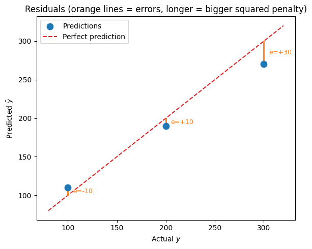

MSE as a Training Objective¶

When training a linear model, the goal is to find the parameter vector $\boldsymbol{\theta}$ that minimises $J$ :

\boldsymbol{\theta}^* = \underset{\boldsymbol{\theta}}{\operatorname{argmin}}\; J(\boldsymbol{\theta})

(7)

In matrix–vector form (the design matrix $\mathbf{X} \in \mathbb{R}^{n \times d}$ , target vector $\mathbf{y} \in \mathbb{R}^n$ ):

J(\boldsymbol{\theta}) = \frac{1}{2} \|\mathbf{y} - \mathbf{X}\boldsymbol{\theta}\|^2

(8)

Setting the gradient to zero and solving yields the Normal Equations:

(\mathbf{X}^\top \mathbf{X})\, \boldsymbol{\theta} = \mathbf{X}^\top \mathbf{y} \quad\Longrightarrow\quad \boldsymbol{\theta}^* = (\mathbf{X}^\top \mathbf{X})^{-1} \mathbf{X}^\top \mathbf{y}

(9)

The gradient descent update rule (preview)¶

Rather than solving the Normal Equations directly, gradient descent iteratively steps toward lower $J$ :

\boldsymbol{\theta} \leftarrow \boldsymbol{\theta} - \alpha\, \nabla_{\boldsymbol{\theta}} J(\boldsymbol{\theta})

(13)

where $\alpha$ is the learning rate. The algorithm repeats until $\|\boldsymbol{\theta}_t - \boldsymbol{\theta}_{t-1}\|$ is below a convergence threshold:

theta, theta_prev = random_initialization()
while norm(theta - theta_prev) > convergence_threshold:
    theta_prev = theta
    theta = theta_prev - step_size * gradient(theta_prev)

Code: Gradient Descent Descending the Loss Curve¶

%matplotlib inline
import numpy as np
import matplotlib.pyplot as plt

np.random.seed(0)
X = np.linspace(0, 10, 100)
true_w = 2.5
y = true_w * X + np.random.normal(0, 2, size=X.shape)

def compute_loss(w):
    return np.mean((y - w * X) ** 2)

def compute_gradient(w):
    return -2 * np.mean(X * (y - w * X))

w_values  = np.linspace(0, 5, 200)
loss_vals = [compute_loss(w) for w in w_values]

w_cur = 0.0
lr    = 0.001
w_hist    = [w_cur]
loss_hist = [compute_loss(w_cur)]
for _ in range(100):
    w_cur -= lr * compute_gradient(w_cur)
    w_hist.append(w_cur)
    loss_hist.append(compute_loss(w_cur))

fig, axes = plt.subplots(1, 2, figsize=(12, 4))

axes[0].plot(w_values, loss_vals, label='Loss curve $J(w)$', color='#1f77b4')
axes[0].scatter(w_hist[::10], loss_hist[::10], color='#d62728', s=40, zorder=5, label='GD steps (every 10th)')
axes[0].axvline(x=true_w, color='#2ca02c', linestyle=':', lw=1.5, label=f'True w={true_w}')
axes[0].set_xlabel('Weight $w$')
axes[0].set_ylabel('MSE $J(w)$')
axes[0].set_title('Gradient Descent on the Loss Surface')
axes[0].legend()

axes[1].plot(loss_hist, color='#ff7f0e')
axes[1].set_xlabel('Iteration')
axes[1].set_ylabel('MSE $J(w)$')
axes[1].set_title('MSE Decreasing During Training')

plt.tight_layout()
plt.show()
print(f"Final learned w = {w_hist[-1]:.4f} (true = {true_w})")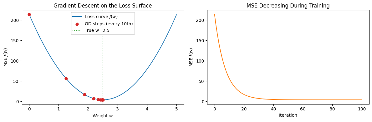

Final learned w = 2.5003 (true = 2.5)

Interactive: Compute MSE in Your Browser¶

Try changing the predicted values below and watch how MSE and RMSE respond.

MSE vs Other Regression Metrics¶

Metric	Formula	Units	Penalises big errors?	Use when
MSE	$\frac{1}{n}\sum e_i^2$	target²	Heavily	Training objective; large-error-sensitive tasks
RMSE	$\sqrt{\text{MSE}}$	target	Heavily	Communicating error magnitude to stakeholders
MAE	$\frac{1}{n}\sum	e_i	$	target
R²	$1 - \frac{\text{SS}_{\text{res}}}{\text{SS}_{\text{tot}}}$	—	N/A	Explaining variance accounted for by the model

Common pitfalls¶

Pitfall	Why it matters
Comparing MSE across datasets with different scales	MSE grows with the magnitude of $y$ — a higher MSE does not always mean a worse model
Reporting MSE without RMSE	MSE is in squared units, making it hard to interpret in meetings
Achieving zero MSE on training data	Perfect training fit usually means overfitting — the model has memorised the data
Ignoring residual plots	MSE gives one number; residual patterns reveal bias, heteroscedasticity, and missed non-linearity

Code: Animated Residuals (Fitting Process)¶

%matplotlib inline
import matplotlib.pyplot as plt
import numpy as np
from matplotlib.animation import FuncAnimation, PillowWriter
from IPython.display import Image

np.random.seed(42)

x_data = np.linspace(0, 10, 20)
y_data = (2 * x_data + 1) + np.random.normal(0, 2, 20)

fig, ax = plt.subplots(figsize=(7, 5))
ax.set_xlim(0, 10)
ax.set_ylim(0, 25)
ax.scatter(x_data, y_data, color='#1f77b4', zorder=5, label='Data points')

line,        = ax.plot([], [], 'r-', lw=2, label='Model line')
error_lines  = [ax.plot([], [], color='#ff7f0e', lw=1.2, linestyle='--')[0] for _ in range(len(x_data))]
loss_text    = ax.text(0.02, 0.95, '', transform=ax.transAxes, va='top', fontsize=9)

def init():
    line.set_data([], [])
    for el in error_lines:
        el.set_data([], [])
    loss_text.set_text('')
    return (line, *error_lines, loss_text)

def animate(i):
    slope     = 0.5 + i * 0.1
    intercept = 0.0 + i * 0.2
    y_pred    = slope * x_data + intercept
    mse_val   = np.mean((y_data - y_pred) ** 2)
    line.set_data(x_data, y_pred)
    for j, el in enumerate(error_lines):
        el.set_data([x_data[j], x_data[j]], [y_data[j], y_pred[j]])
    loss_text.set_text(f'MSE = {mse_val:.1f}')
    return (line, *error_lines, loss_text)

ani = FuncAnimation(fig, animate, frames=np.arange(25), init_func=init, interval=300, blit=True)
ax.legend(loc='upper left', fontsize=8)
ax.set_title('Residuals as the model line sweeps (orange = errors)')
plt.close(fig)  # prevent a static frame appearing alongside the GIF

ani.save('squared_error.gif', writer=PillowWriter(fps=8))
Image(filename='squared_error.gif')

Guided Practice¶

Why does MSE penalise large errors more heavily than MAE?¶

The error term is squared before averaging, so larger residuals contribute quadratically more.Correct. A residual of 10 contributes 100 to MSE, while a residual of 1 contributes only 1 — a 100× difference for a 10× residual difference.

MSE ignores prediction errors near zero.Small errors still contribute to MSE; they are just not amplified as much as large ones.

MSE becomes negative when predictions are too high.Squaring always produces a nonnegative result, so MSE is always ≥ 0.

MSE counts only the single largest residual in the dataset.MSE averages all squared residuals, not just the maximum one.

What does an MSE of zero on the training set indicate?¶

The model has no parameters.Parameter count is unrelated to MSE being zero.

The predictions are uniformly distributed.Uniform predictions would typically produce nonzero error.

Every prediction exactly matches its observed value — a perfect training fit.Correct. Zero squared error across all points means the model passes through every training point. This usually signals overfitting.

All target values in the dataset are identical.Identical targets do not guarantee zero error unless predictions also match.

Why does the MSE cost function often include a $\frac{1}{2}$ factor?¶

It cancels with the exponent during differentiation, keeping the gradient expression tidy.Correct. $\frac{d}{d\theta} \frac{1}{2}e^2 = e$, whereas without the half you get $2e$ — a cosmetic but practically convenient simplification.

It halves the penalty so the model learns more slowly.The $\frac{1}{2}$ does not change which $\theta$ minimises $J$, only the scale of the gradient — which is absorbed by the learning rate.

It converts MSE from squared units to original units.That is what taking the square root (RMSE) does — not multiplying by $\frac{1}{2}$.

It ensures the loss is always between 0 and 1.MSE is unbounded; a $\frac{1}{2}$ factor does not bound it.

Exercises¶

Exercise 1 — Manual MSE Calculation¶

You are forecasting next month’s revenue for four stores:

Store	Actual ($)	Predicted ($)
A	50 000	48 000
B	75 000	80 000
C	60 000	65 000
D	90 000	100 000

Compute MSE and RMSE.
Which store has the largest squared error? What business action might that trigger?
Would you prefer to report MSE or RMSE to your manager, and why?

import numpy as np

y_true = np.array([50000, 75000, 60000, 90000])
y_pred = np.array([48000, 80000, 65000, 100000])

# Your code here
# mse  = ...
# rmse = ...

import numpy as np

y_true = np.array([50000, 75000, 60000, 90000])
y_pred = np.array([48000, 80000, 65000, 100000])

residuals         = y_true - y_pred
squared_residuals = residuals ** 2
mse               = np.mean(squared_residuals)
rmse              = np.sqrt(mse)

stores = ['A', 'B', 'C', 'D']
for s, sq in zip(stores, squared_residuals):
    print(f"Store {s}: squared error = {sq:>15,.0f}")

print(f"\nMSE  = {mse:>15,.0f}")
print(f"RMSE = {rmse:>15,.2f}  (on average off by ~${rmse:,.0f})")

Answers:

MSE ≈ 33,750,000; RMSE ≈ $5,811.
Store D has the largest squared error (100,000²= 10⁹ × 10⁻⁴ → 10,000² = 100,000,000). That 10 % miss on the largest store dominates.
Report RMSE to a manager — “we are off by about $5,800 per store on average” is much more interpretable than a number in squared dollars.

Exercise 2 — Effect of an Outlier¶

Add a fifth store (E) with actual = 100 000, predicted = 200 000 (a catastrophic 100 k miss).

How much does the MSE change?
How does the same outlier affect MAE?
What does this reveal about choosing metrics for a business problem?

import numpy as np

y_true_ext = np.array([50000, 75000, 60000, 90000, 100000])
y_pred_ext = np.array([48000, 80000, 65000, 100000, 200000])

# Compute MSE and MAE with and without the outlier, compare
# Your code here

import numpy as np

y_true_base = np.array([50000, 75000, 60000, 90000])
y_pred_base = np.array([48000, 80000, 65000, 100000])

y_true_ext = np.array([50000, 75000, 60000, 90000, 100000])
y_pred_ext = np.array([48000, 80000, 65000, 100000, 200000])

def report(yt, yp, label):
    mse = np.mean((yt - yp)**2)
    mae = np.mean(np.abs(yt - yp))
    print(f"{label}: MSE={mse:>18,.0f}  MAE={mae:>8,.0f}")

report(y_true_base, y_pred_base, "4 stores (no outlier) ")
report(y_true_ext,  y_pred_ext,  "5 stores (with outlier)")

The single 100 k outlier inflates MSE massively but MAE increases much more moderately. This illustrates why MSE-based training makes the model very sensitive to outliers — which is either a feature or a bug depending on your business context.

Summary¶

Concept	One-line summary
Residual	The gap between an observed value and its prediction: $y^{(i)} - \hat{y}^{(i)}$
MSE	Average squared residual: $\frac{1}{n}\sum_i (y^{(i)} - \hat{y}^{(i)})^2$
Why square?	Eliminates sign; punishes large errors; smooth for calculus
RMSE	$\sqrt{\text{MSE}}$ — same units as target, easier to explain
Training objective	We choose $\boldsymbol{\theta}$ to minimise $J(\boldsymbol{\theta}) = \frac{1}{2n}\|\mathbf{y} - \mathbf{X}\boldsymbol{\theta}\|^2$
Normal Equations	Closed-form solution: $\boldsymbol{\theta}^* = (\mathbf{X}^\top\mathbf{X})^{-1}\mathbf{X}^\top\mathbf{y}$
Sensitivity	MSE is heavily influenced by outliers; MAE is more robust

Next Steps¶

You now know what MSE measures and why it is the right training objective for ordinary least-squares regression. The next notebooks build on this foundation:

regression_metrics.ipynb — full held-out evaluation: RMSE, MAE, R², adjusted R², residual diagnostics.
gradients.ipynb — how gradient descent uses $\nabla J$ to iteratively minimise MSE step by step.
ols.ipynb — the closed-form Normal Equations solution derived in full.