Supervised Regression – Linear Models
Turning numbers into predictions — the foundation of quantitative business analysis

Why Regression Matters in Business

| Business question | Regression answer |
|---|---|
| How much revenue does one extra dollar of ad spend generate? | Coefficient on ad_spend |
| What will next quarter’s sales be? | Predicted from a trained model |
| Which product features drive price? | Coefficients ranked by magnitude |
| How risky is this loan application? | Predicted expected loss |
| Will this marketing channel improve ROI? | Coefficient sign and confidence interval |
The Core Equation
A linear model combines features using a weighted sum:
Color legend: input features learned coefficients intercept
| Symbol | Name | Plain meaning |
|---|---|---|
| Prediction | The number the model outputs | |
| Feature | One measurable input | |
| Coefficient | How much changes per unit change in | |
| Intercept | Baseline prediction when all features are zero |
In matrix form the same equation compresses to:
where is the feature matrix (one row per observation, one column per feature plus a bias column of ones) and is the coefficient vector.
Visual Intuition — How a Linear Model Works
The diagram below traces the lifecycle of a regression model from raw data to a business decision.
Alt: Data enters as a matrix, the model minimises squared errors to learn coefficients, then those coefficients produce predictions that drive decisions.
The cost the model minimises is Mean Squared Error (MSE):
A smaller MSE means predictions stay closer to the actual values. The MSE notebook covers this in depth.
Worked Example — Ad Spend vs Sales
A marketing team collected weekly advertising spend and sales revenue. The question: does spending more on ads reliably lift sales, and by how much?
import pandas as pd
from sklearn.linear_model import LinearRegression
import matplotlib.pyplot as plt

data = pd.DataFrame({
    'Ad_Spend': [100, 200, 300, 400, 500, 600, 700],
    'Sales':    [12,  22,  26,  36,  44,  52,  60]
})

X = data[['Ad_Spend']]
y = data['Sales']

model = LinearRegression().fit(X, y)
print(f"Coefficient (slope):  {model.coef_[0]:.4f}  → each £1 extra spend → £{model.coef_[0]:.4f}k extra sales")
print(f"Intercept (baseline): {model.intercept_:.2f}")
print(f"R² on training data:  {model.score(X, y):.4f}")

# Plot
fig, ax = plt.subplots(figsize=(7, 4))
ax.scatter(data['Ad_Spend'], data['Sales'], color='#1d4ed8', s=60, label='Actual data', zorder=3)
ax.plot(data['Ad_Spend'], model.predict(X), color='#b91c1c', lw=2, label='Fitted line')
ax.set_xlabel('Advertising Spend (£)')
ax.set_ylabel('Sales (£ thousands)')
ax.set_title('Linear Regression: Ad Spend → Sales')
ax.legend()
plt.tight_layout()
plt.show()
Coefficient (slope): 0.0793 → each £1 extra spend → £0.0793k extra sales
Intercept (baseline): 4.29
R² on training data: 0.9956
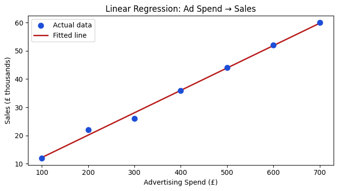
Interpret the result
A coefficient of roughly 0.08 means every additional £1 of advertising spend is associated with £0.08k (£80) of additional sales — a rough 8 % return per pound spent at this scale. The intercept of about 4 means the model predicts ~£4k sales even with zero ad spend, which may reflect baseline organic demand.
The close to 1.0 on this small dataset tells us the line fits well, but we should always evaluate on held-out data before trusting the estimate.
Key Assumptions
Linear regression relies on four main assumptions. Violating them does not always break the model, but it does limit what you can safely conclude.
| Assumption | If violated | Practical check |
|---|---|---|
| Linearity | Model underfits curved patterns | Residual vs fitted plot — look for curves |
| Independence | Standard errors are wrong | Time or group structure in residuals |
| Homoscedasticity | Confidence intervals are unreliable | Residual spread widens with fitted values |
| Low multicollinearity | Coefficients become unstable | Variance Inflation Factor (VIF) > 10 |
Interactive — Explore Slope and Intercept
Use the Pyodide cell below to change the coefficient (slope) and intercept values and observe how the predicted line shifts. This builds intuition before you move to fitting from real data.
What to notice
A higher slope makes the line steeper — predictions grow faster as spend increases.
A higher intercept shifts the whole line up — the baseline prediction increases.
MSE decreases as your hand-tuned values approach what
LinearRegression().fit()finds automatically.OLS (Ordinary Least Squares) finds the slope and intercept that minimise MSE exactly — covered in the OLS notebook.
Chapter Map
This chapter is a parent section. Each child notebook covers one focused topic. Use the map below to navigate.
Suggested reading order: Linear Model Family → MSE → Metrics → Gradients → OLS → Polynomial → Regularization → Bias–Variance → Lab.
Guided Practice
What kind of output does a regression model produce?
A coefficient of 0.09 on an "ad_spend" feature means:
Which assumption is most likely violated when a residual plot shows a funnel shape (small spread on the left, large spread on the right)?
Exercises
Exercise 1 — Interpret a coefficient
A model trained on house price data returns:
Intercept: 50,000
Coefficient on
floor_area_sqm: 2,500Coefficient on
distance_to_station_km: -8,000
Answer in plain language: (a) What does the model predict for a 100 sqm house 1 km from a station? (b) What does the negative coefficient on distance mean for a business selling property near commuter hubs?
Hint
Plug the values into directly. For the business interpretation, think about what a negative coefficient on distance implies: closer is better (higher price), so the coefficient captures the premium for proximity.
Model answer
(a)
(b) Each extra kilometre from a station is associated with an £8,000 drop in predicted price. This tells a developer to pay a premium for sites within walking distance of stations, as the market prices in that convenience.
Exercise 2 — Fit and plot from data
Use the dataset below. Fit a linear regression, print the coefficient and intercept, plot the fitted line, and calculate .
import pandas as pd
from sklearn.linear_model import LinearRegression

df = pd.DataFrame({
    'store_size_sqm': [200, 350, 500, 650, 800, 950, 1100],
    'weekly_revenue': [8000, 13500, 18000, 23500, 28000, 33000, 38500]
})

# TODO: Fit LinearRegression, print coefficient, intercept, R²
# TODO: Plot scatter + fitted line
Model solution
import matplotlib.pyplot as plt

X = df[['store_size_sqm']]
y = df['weekly_revenue']
model = LinearRegression().fit(X, y)

print(f"Coefficient: {model.coef_[0]:.2f}")
print(f"Intercept:   {model.intercept_:.2f}")
print(f"R²:          {model.score(X, y):.4f}")

fig, ax = plt.subplots(figsize=(6, 4))
ax.scatter(df['store_size_sqm'], df['weekly_revenue'], color='#1d4ed8', label='Actual')
ax.plot(df['store_size_sqm'], model.predict(X), color='#b91c1c', lw=2, label='Fitted')
ax.set_xlabel('Store Size (sqm)')
ax.set_ylabel('Weekly Revenue (£)')
ax.legend()
plt.tight_layout()
plt.show()
Interpretation: A coefficient near 35 means each extra square metre is associated with roughly £35 of additional weekly revenue. close to 1.0 on this synthetic dataset confirms the linear fit is excellent.
Summary
Key takeaways
Regression predicts continuous values — revenue, price, risk, demand — not categories.
Coefficients are the core insight: each one tells you how much the prediction changes per unit change in that feature.
The model minimises MSE to find the best-fitting coefficients.
Four assumptions underpin valid inference: linearity, independence, constant variance, and low multicollinearity. Always check residuals.
Matrix form connects what you learned in linear algebra directly to the regression equation.
Next Steps
The next notebook — Linear Model Family — maps out the full family of linear models: simple regression with one feature, multiple regression with many features, interaction terms, and generalised linear models. Start there to build a complete picture before diving into the MSE objective, gradient derivation, or regularization.