Bias–Variance Tradeoff¶

The Fundamental Tension in Every Model¶

Every model makes a choice: be simple and predictable, or be flexible and expressive. Push too far in either direction and generalisation suffers. This notebook gives you the mathematical decomposition of error, the tools to diagnose which problem you have, and the practical levers to fix it.

Intuition — The Bullseye Analogy¶

Imagine shooting arrows at a target:

Pattern	Bias	Variance	Meaning
All arrows clustered, but off-centre	High	Low	Consistently wrong — underfitting
Arrows scattered everywhere	Low	High	Unpredictable — overfitting
All arrows near centre	Low	Low	The goal
Arrows scattered AND off-centre	High	High	Worst case

Bias = systematic error — the model consistently misses in the same direction because it is too simple to capture the true pattern.
Variance = instability — the model’s predictions shift a lot depending on which training samples it saw.
Irreducible error = the noise floor in the data itself; no model can eliminate it.

Mathematical Decomposition¶

For a regression problem with true function $f(x)$ and noise $\epsilon \sim \mathcal{N}(0, \sigma^2)$ :

y = f(x) + \epsilon

(1)

The expected test MSE at a point $x_0$ , averaged over all possible training sets $\mathcal{D}$ , decomposes as:

\underbrace{\mathbb{E}_{\mathcal{D}}\left[(y_0 - \hat{f}(x_0))^2\right]}_{\text{Expected test MSE}} = \underbrace{\left(f(x_0) - \mathbb{E}_{\mathcal{D}}[\hat{f}(x_0)]\right)^2}_{\text{Bias}^2} + \underbrace{\mathbb{E}_{\mathcal{D}}\left[\left(\hat{f}(x_0) - \mathbb{E}_{\mathcal{D}}[\hat{f}(x_0)]\right)^2\right]}_{\text{Variance}} + \underbrace{\sigma^2}_{\text{Irreducible error}}

(2)

Term	Formula	Meaning
$\text{Bias}^2$	$(f(x_0) - \mathbb{E}[\hat{f}])^2$	How far the average prediction is from truth
$\text{Variance}$	$\mathbb{E}[(\hat{f} - \mathbb{E}[\hat{f}])^2]$	How much predictions scatter across training sets
$\sigma^2$	$\mathbb{E}[(y - f)^2]$	Irreducible noise — cannot be reduced

The U-Shaped Error Curve¶

As model complexity increases:

$\text{Bias}^2$ decreases (the model can represent more patterns)
$\text{Variance}$ increases (the model becomes more sensitive to its specific training data)
Total error = $\text{Bias}^2 + \text{Variance} + \sigma^2$ forms a U-shape — there is an optimal complexity in the middle.

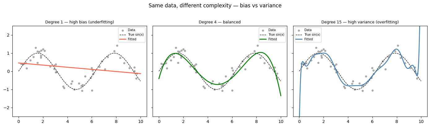
Visualising the Tradeoff — Model Fits at Different Complexities¶

%matplotlib inline
import numpy as np
import matplotlib.pyplot as plt
from sklearn.preprocessing import PolynomialFeatures, StandardScaler
from sklearn.linear_model import LinearRegression
from sklearn.pipeline import make_pipeline

np.random.seed(42)
n = 50
X_all = np.sort(np.random.rand(n) * 10).reshape(-1, 1)
y_all = np.sin(X_all).ravel() + np.random.randn(n) * 0.3

X_plot = np.linspace(0, 10, 300).reshape(-1, 1)
y_true = np.sin(X_plot).ravel()

degrees = [1, 4, 15]
labels  = ['Degree 1 — high bias (underfitting)',
           'Degree 4 — balanced',
           'Degree 15 — high variance (overfitting)']
colors  = ['tomato', 'green', 'steelblue']

fig, axes = plt.subplots(1, 3, figsize=(14, 4), sharey=True)
for ax, degree, label, color in zip(axes, degrees, labels, colors):
    pipe = make_pipeline(PolynomialFeatures(degree), StandardScaler(), LinearRegression())
    pipe.fit(X_all, y_all)
    ax.scatter(X_all, y_all, color='grey', s=15, alpha=0.6, label='Data')
    ax.plot(X_plot, y_true, 'k--', linewidth=1, label='True sin(x)')
    ax.plot(X_plot, np.clip(pipe.predict(X_plot), -3, 3), color=color, linewidth=2, label='Fitted')
    ax.set_title(label, fontsize=9)
    ax.set_ylim(-2.5, 2.5)
    ax.legend(fontsize=7)

plt.suptitle('Same data, different complexity — bias vs variance', y=1.02)
plt.tight_layout()
plt.show()

/Volumes/MacSSD/01_Projects/Chandravesh-ML-Research/projects/jupyter-books/.venv/lib/python3.10/site-packages/sklearn/linear_model/_base.py:280: RuntimeWarning: divide by zero encountered in matmul
  return X @ coef_ + self.intercept_
/Volumes/MacSSD/01_Projects/Chandravesh-ML-Research/projects/jupyter-books/.venv/lib/python3.10/site-packages/sklearn/linear_model/_base.py:280: RuntimeWarning: overflow encountered in matmul
  return X @ coef_ + self.intercept_
/Volumes/MacSSD/01_Projects/Chandravesh-ML-Research/projects/jupyter-books/.venv/lib/python3.10/site-packages/sklearn/linear_model/_base.py:280: RuntimeWarning: invalid value encountered in matmul
  return X @ coef_ + self.intercept_
/Volumes/MacSSD/01_Projects/Chandravesh-ML-Research/projects/jupyter-books/.venv/lib/python3.10/site-packages/sklearn/linear_model/_base.py:280: RuntimeWarning: divide by zero encountered in matmul
  return X @ coef_ + self.intercept_
/Volumes/MacSSD/01_Projects/Chandravesh-ML-Research/projects/jupyter-books/.venv/lib/python3.10/site-packages/sklearn/linear_model/_base.py:280: RuntimeWarning: overflow encountered in matmul
  return X @ coef_ + self.intercept_
/Volumes/MacSSD/01_Projects/Chandravesh-ML-Research/projects/jupyter-books/.venv/lib/python3.10/site-packages/sklearn/linear_model/_base.py:280: RuntimeWarning: invalid value encountered in matmul
  return X @ coef_ + self.intercept_

Empirical Decomposition — Bootstrapping Bias and Variance¶

We can estimate bias and variance empirically by training the model on many bootstrap samples and observing how predictions scatter.

%matplotlib inline
import numpy as np
import matplotlib.pyplot as plt
from sklearn.preprocessing import PolynomialFeatures, StandardScaler
from sklearn.linear_model import LinearRegression
from sklearn.pipeline import make_pipeline

def true_func(x):
    return np.sin(x)

rng = np.random.default_rng(7)
n_train = 40
n_boot  = 80
X_train = np.sort(rng.uniform(0, 10, n_train)).reshape(-1, 1)
X_eval  = np.linspace(0, 10, 200).reshape(-1, 1)
y_true_eval = true_func(X_eval.ravel())

degrees = [1, 3, 5, 10, 20]
bias2_list, var_list, total_list = [], [], []

for degree in degrees:
    preds_boot = np.zeros((n_boot, len(X_eval)))
    for b in range(n_boot):
        idx = rng.integers(0, n_train, n_train)
        Xb  = X_train[idx]
        yb  = true_func(Xb.ravel()) + rng.normal(0, 0.3, n_train)
        pipe = make_pipeline(PolynomialFeatures(degree), StandardScaler(), LinearRegression())
        pipe.fit(Xb, yb)
        preds_boot[b] = pipe.predict(X_eval)
    mean_pred = preds_boot.mean(axis=0)
    b2 = np.mean((mean_pred - y_true_eval) ** 2)
    v  = np.mean(preds_boot.var(axis=0))
    bias2_list.append(b2)
    var_list.append(v)
    total_list.append(b2 + v + 0.09)   # 0.09 = sigma^2 = 0.3^2

fig, ax = plt.subplots(figsize=(9, 5))
ax.plot(degrees, bias2_list,  'b-o', linewidth=2, label=r'Bias$^2$')
ax.plot(degrees, var_list,    'r-o', linewidth=2, label='Variance')
ax.plot(degrees, total_list,  'g-o', linewidth=2, label=r'Bias$^2$ + Var + $\sigma^2$')
ax.set_xlabel('Polynomial degree')
ax.set_ylabel('Error component')
ax.set_title('Empirical bias-variance decomposition via bootstrapping')
ax.legend()
ax.grid(True, alpha=0.3)
plt.tight_layout()
plt.show()

print(f"{'Degree':>6}  {'Bias2':>8}  {'Variance':>10}  {'Total':>8}")
for d, b2, v, t in zip(degrees, bias2_list, var_list, total_list):
    print(f"{d:>6}  {b2:>8.4f}  {v:>10.4f}  {t:>8.4f}")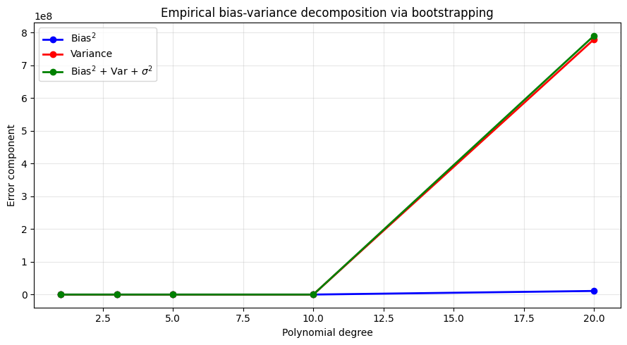

Fetching long content....

Degree     Bias2    Variance     Total
     1    0.4410      0.0218    0.5528
     3    0.3814      0.1225    0.5939
     5    0.0373      0.0416    0.1689
    10    0.1265     10.7161   10.9327
    20  10976269.8496  779420743.7784  790397013.7179

Learning Curves — Diagnosing Bias vs Variance¶

A learning curve plots train and validation error against training set size. The pattern reveals which problem dominates.

%matplotlib inline
import numpy as np
import matplotlib.pyplot as plt
from sklearn.preprocessing import PolynomialFeatures, StandardScaler
from sklearn.linear_model import LinearRegression
from sklearn.pipeline import make_pipeline
from sklearn.model_selection import learning_curve

np.random.seed(0)
n = 100
X = np.sort(np.random.rand(n) * 10).reshape(-1, 1)
y = np.sin(X).ravel() + np.random.randn(n) * 0.5

def plot_lc(degree, ax, title):
    pipe = make_pipeline(PolynomialFeatures(degree), StandardScaler(), LinearRegression())
    sizes, tr_sc, val_sc = learning_curve(
        pipe, X, y, cv=5,
        scoring='neg_mean_squared_error',
        train_sizes=np.linspace(0.1, 1.0, 8)
    )
    tr_mse  = -tr_sc.mean(axis=1)
    val_mse = -val_sc.mean(axis=1)
    ax.plot(sizes, tr_mse,  'b-o', linewidth=2, markersize=5, label='Training MSE')
    ax.plot(sizes, val_mse, 'r-o', linewidth=2, markersize=5, label='Validation MSE')
    ax.set_title(title, fontsize=10)
    ax.set_xlabel('Training set size')
    ax.set_ylabel('MSE')
    ax.legend(fontsize=8)
    ax.grid(True, alpha=0.3)
    return tr_mse[-1], val_mse[-1]

fig, axes = plt.subplots(1, 2, figsize=(12, 5))
tr1, v1 = plot_lc(1,  axes[0], 'Degree 1 — High Bias (Underfitting)')
tr15, v15 = plot_lc(15, axes[1], 'Degree 15 — High Variance (Overfitting)')
plt.suptitle('Learning curves reveal the dominant problem', y=1.02)
plt.tight_layout()
plt.show()

print(f'Degree  1:  train MSE={tr1:.3f}  val MSE={v1:.3f}  gap={v1-tr1:.3f}')
print(f'Degree 15:  train MSE={tr15:.3f}  val MSE={v15:.3f}  gap={v15-tr15:.3f}')

/Volumes/MacSSD/01_Projects/Chandravesh-ML-Research/projects/jupyter-books/.venv/lib/python3.10/site-packages/sklearn/linear_model/_base.py:280: RuntimeWarning: divide by zero encountered in matmul
  return X @ coef_ + self.intercept_
/Volumes/MacSSD/01_Projects/Chandravesh-ML-Research/projects/jupyter-books/.venv/lib/python3.10/site-packages/sklearn/linear_model/_base.py:280: RuntimeWarning: overflow encountered in matmul
  return X @ coef_ + self.intercept_
/Volumes/MacSSD/01_Projects/Chandravesh-ML-Research/projects/jupyter-books/.venv/lib/python3.10/site-packages/sklearn/linear_model/_base.py:280: RuntimeWarning: invalid value encountered in matmul
  return X @ coef_ + self.intercept_
/Volumes/MacSSD/01_Projects/Chandravesh-ML-Research/projects/jupyter-books/.venv/lib/python3.10/site-packages/sklearn/linear_model/_base.py:280: RuntimeWarning: divide by zero encountered in matmul
  return X @ coef_ + self.intercept_
/Volumes/MacSSD/01_Projects/Chandravesh-ML-Research/projects/jupyter-books/.venv/lib/python3.10/site-packages/sklearn/linear_model/_base.py:280: RuntimeWarning: overflow encountered in matmul
  return X @ coef_ + self.intercept_
/Volumes/MacSSD/01_Projects/Chandravesh-ML-Research/projects/jupyter-books/.venv/lib/python3.10/site-packages/sklearn/linear_model/_base.py:280: RuntimeWarning: invalid value encountered in matmul
  return X @ coef_ + self.intercept_
/Volumes/MacSSD/01_Projects/Chandravesh-ML-Research/projects/jupyter-books/.venv/lib/python3.10/site-packages/sklearn/linear_model/_base.py:280: RuntimeWarning: divide by zero encountered in matmul
  return X @ coef_ + self.intercept_
/Volumes/MacSSD/01_Projects/Chandravesh-ML-Research/projects/jupyter-books/.venv/lib/python3.10/site-packages/sklearn/linear_model/_base.py:280: RuntimeWarning: overflow encountered in matmul
  return X @ coef_ + self.intercept_
/Volumes/MacSSD/01_Projects/Chandravesh-ML-Research/projects/jupyter-books/.venv/lib/python3.10/site-packages/sklearn/linear_model/_base.py:280: RuntimeWarning: invalid value encountered in matmul
  return X @ coef_ + self.intercept_
/Volumes/MacSSD/01_Projects/Chandravesh-ML-Research/projects/jupyter-books/.venv/lib/python3.10/site-packages/sklearn/linear_model/_base.py:280: RuntimeWarning: divide by zero encountered in matmul
  return X @ coef_ + self.intercept_
/Volumes/MacSSD/01_Projects/Chandravesh-ML-Research/projects/jupyter-books/.venv/lib/python3.10/site-packages/sklearn/linear_model/_base.py:280: RuntimeWarning: overflow encountered in matmul
  return X @ coef_ + self.intercept_
/Volumes/MacSSD/01_Projects/Chandravesh-ML-Research/projects/jupyter-books/.venv/lib/python3.10/site-packages/sklearn/linear_model/_base.py:280: RuntimeWarning: invalid value encountered in matmul
  return X @ coef_ + self.intercept_
/Volumes/MacSSD/01_Projects/Chandravesh-ML-Research/projects/jupyter-books/.venv/lib/python3.10/site-packages/sklearn/linear_model/_base.py:280: RuntimeWarning: divide by zero encountered in matmul
  return X @ coef_ + self.intercept_
/Volumes/MacSSD/01_Projects/Chandravesh-ML-Research/projects/jupyter-books/.venv/lib/python3.10/site-packages/sklearn/linear_model/_base.py:280: RuntimeWarning: overflow encountered in matmul
  return X @ coef_ + self.intercept_
/Volumes/MacSSD/01_Projects/Chandravesh-ML-Research/projects/jupyter-books/.venv/lib/python3.10/site-packages/sklearn/linear_model/_base.py:280: RuntimeWarning: invalid value encountered in matmul
  return X @ coef_ + self.intercept_

/Volumes/MacSSD/01_Projects/Chandravesh-ML-Research/projects/jupyter-books/.venv/lib/python3.10/site-packages/sklearn/linear_model/_base.py:280: RuntimeWarning: divide by zero encountered in matmul
  return X @ coef_ + self.intercept_
/Volumes/MacSSD/01_Projects/Chandravesh-ML-Research/projects/jupyter-books/.venv/lib/python3.10/site-packages/sklearn/linear_model/_base.py:280: RuntimeWarning: overflow encountered in matmul
  return X @ coef_ + self.intercept_
/Volumes/MacSSD/01_Projects/Chandravesh-ML-Research/projects/jupyter-books/.venv/lib/python3.10/site-packages/sklearn/linear_model/_base.py:280: RuntimeWarning: invalid value encountered in matmul
  return X @ coef_ + self.intercept_
/Volumes/MacSSD/01_Projects/Chandravesh-ML-Research/projects/jupyter-books/.venv/lib/python3.10/site-packages/sklearn/linear_model/_base.py:280: RuntimeWarning: divide by zero encountered in matmul
  return X @ coef_ + self.intercept_
/Volumes/MacSSD/01_Projects/Chandravesh-ML-Research/projects/jupyter-books/.venv/lib/python3.10/site-packages/sklearn/linear_model/_base.py:280: RuntimeWarning: overflow encountered in matmul
  return X @ coef_ + self.intercept_
/Volumes/MacSSD/01_Projects/Chandravesh-ML-Research/projects/jupyter-books/.venv/lib/python3.10/site-packages/sklearn/linear_model/_base.py:280: RuntimeWarning: invalid value encountered in matmul
  return X @ coef_ + self.intercept_
/Volumes/MacSSD/01_Projects/Chandravesh-ML-Research/projects/jupyter-books/.venv/lib/python3.10/site-packages/sklearn/linear_model/_base.py:280: RuntimeWarning: divide by zero encountered in matmul
  return X @ coef_ + self.intercept_
/Volumes/MacSSD/01_Projects/Chandravesh-ML-Research/projects/jupyter-books/.venv/lib/python3.10/site-packages/sklearn/linear_model/_base.py:280: RuntimeWarning: overflow encountered in matmul
  return X @ coef_ + self.intercept_
/Volumes/MacSSD/01_Projects/Chandravesh-ML-Research/projects/jupyter-books/.venv/lib/python3.10/site-packages/sklearn/linear_model/_base.py:280: RuntimeWarning: invalid value encountered in matmul
  return X @ coef_ + self.intercept_
/Volumes/MacSSD/01_Projects/Chandravesh-ML-Research/projects/jupyter-books/.venv/lib/python3.10/site-packages/sklearn/linear_model/_base.py:280: RuntimeWarning: divide by zero encountered in matmul
  return X @ coef_ + self.intercept_
/Volumes/MacSSD/01_Projects/Chandravesh-ML-Research/projects/jupyter-books/.venv/lib/python3.10/site-packages/sklearn/linear_model/_base.py:280: RuntimeWarning: overflow encountered in matmul
  return X @ coef_ + self.intercept_
/Volumes/MacSSD/01_Projects/Chandravesh-ML-Research/projects/jupyter-books/.venv/lib/python3.10/site-packages/sklearn/linear_model/_base.py:280: RuntimeWarning: invalid value encountered in matmul
  return X @ coef_ + self.intercept_
/Volumes/MacSSD/01_Projects/Chandravesh-ML-Research/projects/jupyter-books/.venv/lib/python3.10/site-packages/sklearn/linear_model/_base.py:280: RuntimeWarning: divide by zero encountered in matmul
  return X @ coef_ + self.intercept_
/Volumes/MacSSD/01_Projects/Chandravesh-ML-Research/projects/jupyter-books/.venv/lib/python3.10/site-packages/sklearn/linear_model/_base.py:280: RuntimeWarning: overflow encountered in matmul
  return X @ coef_ + self.intercept_
/Volumes/MacSSD/01_Projects/Chandravesh-ML-Research/projects/jupyter-books/.venv/lib/python3.10/site-packages/sklearn/linear_model/_base.py:280: RuntimeWarning: invalid value encountered in matmul
  return X @ coef_ + self.intercept_

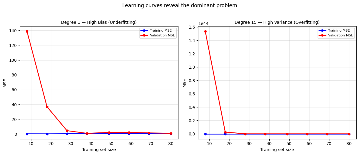
Degree  1:  train MSE=0.646  val MSE=1.057  gap=0.412
Degree 15:  train MSE=0.204  val MSE=1874086326.573  gap=1874086326.369

How to read learning curves

Pattern	Diagnosis	Fix
Both curves high and close together	High bias — underfitting	Increase complexity; add features
Large gap between train and val	High variance — overfitting	More data; regularise; reduce complexity
Val curve still falling as n grows	Variance-limited	Collect more training data
Val curve flat regardless of n	Bias-limited	Model needs more expressive power

Train vs Test Error Across Model Complexity¶

%matplotlib inline
import numpy as np
import matplotlib.pyplot as plt
from sklearn.preprocessing import PolynomialFeatures, StandardScaler
from sklearn.linear_model import LinearRegression
from sklearn.pipeline import make_pipeline
from sklearn.model_selection import train_test_split
from sklearn.metrics import mean_squared_error

np.random.seed(42)
n = 80
X = np.sort(np.random.rand(n) * 10).reshape(-1, 1)
y = np.sin(X).ravel() + np.random.randn(n) * 0.4
X_tr, X_te, y_tr, y_te = train_test_split(X, y, test_size=0.25, random_state=0)

degrees = list(range(1, 18))
tr_errs, te_errs = [], []
for d in degrees:
    pipe = make_pipeline(PolynomialFeatures(d), StandardScaler(), LinearRegression())
    pipe.fit(X_tr, y_tr)
    tr_errs.append(mean_squared_error(y_tr, pipe.predict(X_tr)))
    te_errs.append(mean_squared_error(y_te, pipe.predict(X_te)))

best_d = degrees[np.argmin(te_errs)]

fig, ax = plt.subplots(figsize=(10, 5))
ax.plot(degrees, tr_errs, 'b-o', linewidth=2, markersize=5, label='Training MSE')
ax.plot(degrees, te_errs, 'r-o', linewidth=2, markersize=5, label='Test MSE')
ax.axvline(best_d, color='green', linestyle='--', linewidth=1.5, label=f'Best degree ({best_d})')
ax.set_xlabel('Polynomial degree')
ax.set_ylabel('MSE')
ax.set_title('Train MSE always falls; test MSE forms a U-shape')
ax.legend()
ax.grid(True, alpha=0.3)
plt.tight_layout()
plt.show()

print(f'Optimal degree by test MSE: {best_d}')

/Volumes/MacSSD/01_Projects/Chandravesh-ML-Research/projects/jupyter-books/.venv/lib/python3.10/site-packages/sklearn/linear_model/_base.py:280: RuntimeWarning: divide by zero encountered in matmul
  return X @ coef_ + self.intercept_
/Volumes/MacSSD/01_Projects/Chandravesh-ML-Research/projects/jupyter-books/.venv/lib/python3.10/site-packages/sklearn/linear_model/_base.py:280: RuntimeWarning: overflow encountered in matmul
  return X @ coef_ + self.intercept_
/Volumes/MacSSD/01_Projects/Chandravesh-ML-Research/projects/jupyter-books/.venv/lib/python3.10/site-packages/sklearn/linear_model/_base.py:280: RuntimeWarning: invalid value encountered in matmul
  return X @ coef_ + self.intercept_

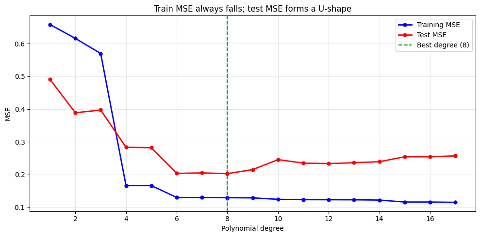
Optimal degree by test MSE: 8

Regularisation as a Variance Reducer¶

Regularisation does not reduce irreducible error $\sigma^2$ , but it does reduce variance by constraining coefficients:

%matplotlib inline
import numpy as np
import matplotlib.pyplot as plt
from sklearn.linear_model import Ridge
from sklearn.preprocessing import PolynomialFeatures, StandardScaler
from sklearn.pipeline import make_pipeline

def true_func(x): return np.sin(x)

rng = np.random.default_rng(3)
n_boot = 50
X_eval = np.linspace(0, 10, 200).reshape(-1, 1)
y_true = true_func(X_eval.ravel())

fig, axes = plt.subplots(1, 2, figsize=(13, 5), sharey=True)
for ax, alpha, title in [(axes[0], 0.0, 'No regularisation — high variance'),
                          (axes[1], 5.0, 'Ridge alpha=5 — variance reduced')]:
    ax.plot(X_eval, y_true, 'k-', linewidth=2, label='True function', zorder=5)
    all_preds = []
    for _ in range(n_boot):
        n_tr = 30
        Xb = np.sort(rng.uniform(0, 10, n_tr)).reshape(-1, 1)
        yb = true_func(Xb.ravel()) + rng.normal(0, 0.5, n_tr)
        pipe = make_pipeline(PolynomialFeatures(12), StandardScaler(),
                             Ridge(alpha=alpha if alpha > 0 else 1e-10))
        pipe.fit(Xb, yb)
        pred = np.clip(pipe.predict(X_eval), -3, 3)
        all_preds.append(pred)
        ax.plot(X_eval, pred, 'steelblue', alpha=0.12, linewidth=0.8)
    mean_pred = np.array(all_preds).mean(axis=0)
    ax.plot(X_eval, mean_pred, 'orange', linewidth=2.5, label='Mean prediction')
    ax.set_title(title)
    ax.set_ylim(-2.5, 2.5)
    ax.legend(fontsize=8)

plt.suptitle('Degree-12 polynomial: 50 bootstrap fits', y=1.02)
plt.tight_layout()
plt.show()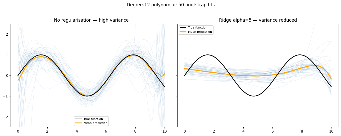

Fetching long content....

Try It in the Browser¶

Compute bias and variance manually from a list of bootstrap predictions.

Practical Levers¶

Action	Reduces bias	Reduces variance	Notes
Increase model complexity	Yes	No — increases it	Use carefully; pair with regularisation
Add regularisation (Ridge/Lasso)	No	Yes	The main tool from the previous notebook
Collect more training data	No	Yes	Most reliable variance fix
Add informative features	Yes	Slightly	Domain knowledge matters
Feature selection / dimensionality reduction	Slightly	Yes	Removes noise dimensions
Ensemble methods (bagging)	No	Yes	Average many high-variance models
Ensemble methods (boosting)	Yes	Slightly	Stack many high-bias models

Guided Practice¶

What usually happens when model bias is high?¶

The model is too simple and underfits the dataCorrect. High bias means the model's assumptions are too restrictive to capture the true pattern.

The model memorises every training example perfectlyThat is high variance (overfitting), not high bias.

The evaluation metric becomes undefinedBias does not automatically invalidate metrics.

The learning rate must be reducedLearning rate affects optimisation speed; it is not the definition of bias.

What usually indicates high variance?¶

The model performs equally poorly on training and test dataEqual performance (both poor) is the signature of high bias / underfitting.

The model fits training data well but generalises poorly to new dataCorrect. High variance means predictions are overly sensitive to the specific training sample.

The target variable becomes categoricalVariance is unrelated to the type of target variable.

The gradient always equals zeroA zero gradient indicates convergence; it is not the definition of high variance.

Collecting more training data primarily helps with which problem?¶

High biasMore data does not fix a model that is too simple to represent the pattern. You need higher complexity.

High varianceCorrect. More data exposes the model to more of the distribution, reducing its sensitivity to any one training sample.

Irreducible errorIrreducible error is noise in the data that no amount of data can eliminate.

Both bias and variance equallyMore data primarily helps variance. It does very little for a fundamentally too-simple model.

On a learning curve, you see that both training and validation MSE are high and barely converge as you add more data. What does this indicate?¶

High variance — collect more dataHigh variance shows a large gap between train and validation error, not both being high together.

High bias — increase model complexity or add featuresCorrect. When both curves converge at a high error level, the model is too simple regardless of data size.

The data is corruptedCorrupted data is not the typical interpretation of this learning curve pattern.

The learning rate is too highLearning rate affects optimisation convergence, not the learning curve pattern described.

Exercises¶

Exercise 1 — Compute the decomposition¶

Run 50 bootstrap iterations for degree-1, degree-5, and degree-12 polynomial fits on the same dataset. Print a table of $\text{Bias}^2$ , $\text{Variance}$ , and total estimated MSE for each degree.

%matplotlib inline
import numpy as np
from sklearn.preprocessing import PolynomialFeatures, StandardScaler
from sklearn.linear_model import LinearRegression
from sklearn.pipeline import make_pipeline

rng = np.random.default_rng(42)
n_train = 30
n_boot  = 50
sigma2  = 0.16   # assumed noise variance

X_eval   = np.linspace(0, 10, 150).reshape(-1, 1)
y_true   = np.sin(X_eval.ravel())

# TODO: for each degree in [1, 5, 12]:
#   run n_boot bootstrap fits
#   compute mean prediction over bootstraps
#   compute bias^2 and variance
#   print a summary table

for degree in [1, 5, 12]:
    preds = []
    for _ in range(n_boot):
        idx = rng.integers(0, n_train, n_train)
        Xb = np.sort(rng.uniform(0, 10, n_train)).reshape(-1, 1)
        yb = np.sin(Xb.ravel()) + rng.normal(0, 0.4, n_train)
        pipe = make_pipeline(PolynomialFeatures(degree), StandardScaler(), LinearRegression())
        pipe.fit(Xb, yb)
        preds.append(pipe.predict(X_eval))
    preds = np.array(preds)
    mean_p = preds.mean(0)
    bias2 = np.mean((mean_p - y_true)**2)
    var   = np.mean(preds.var(0))
    print(f"d={degree}  bias2={bias2:.4f}  var={var:.4f}  total={bias2+var+sigma2:.4f}")

Exercise 2 — Effect of training size on variance¶

Fix degree=10. Run the bootstrap decomposition for training sizes [10, 20, 40, 80, 160]. Plot $\text{Bias}^2$ and $\text{Variance}$ vs training size and describe what you observe.

# Your code here

Exercise 3 — Regularisation as a variance reducer¶

Fix degree=12. Run the bootstrap decomposition for Ridge with alpha in [0, 0.1, 1, 10, 100]. Plot how $\text{Bias}^2$ , $\text{Variance}$ , and total error change as $\alpha$ increases. Explain the tradeoff in 2–3 sentences.

# Your code here

Common Pitfalls¶

Summary¶

Concept	One-line meaning
Bias	Systematic gap between average prediction and truth — underfitting
Variance	Prediction instability across training sets — overfitting
Irreducible error	Noise floor $\sigma^2$ — no model can beat it
Decomposition	$\text{Expected test MSE} = \text{Bias}^2 + \text{Variance} + \sigma^2$
U-shape	Total error has a minimum at the optimal complexity
Learning curve	Plots train/val error vs data size — diagnoses which problem dominates
Fix bias	Increase complexity; add features; reduce regularisation
Fix variance	More data; regularise; reduce complexity; use ensembles

Next Up — Cross-Validation¶

You can now diagnose bias vs variance. Next: measure generalisation reliably.¶

The next notebook — Cross-Validation — shows how to estimate test error without wasting data on a fixed holdout set. $k$-fold CV, stratified splits, leave-one-out, and nested CV for hyperparameter tuning all rest on the ideas you just learned about train vs validation error.

Dependencies you already have: train/test split intuition, MSE as evaluation metric, and the insight that a model's test error is the sum of bias, variance, and irreducible noise.