Naive Bayes¶

Learning objectives

By the end of this notebook you will be able to:

Apply Bayes’ theorem to derive the posterior class probability from a likelihood and a prior.
Explain the naive conditional independence assumption and why it works in practice.
Implement Gaussian Naive Bayes from scratch using MLE parameter estimation.
Implement Multinomial Naive Bayes with Laplace smoothing for text classification.
Distinguish when to use Gaussian vs Multinomial vs Bernoulli NB.
Compare Naive Bayes (generative) to Logistic Regression (discriminative).
Apply Multinomial NB to spam classification using a bag-of-words representation.
Recognise the zero-frequency problem and fix it with Laplace smoothing.

Business hook — Spam in 4 microseconds¶

Gmail classifies billions of emails a day. It needs a classifier that is fast to train, fast to predict, and handles millions of word features gracefully. Naive Bayes was the algorithm that powered early spam filters and still runs inside many production text classifiers — not because the independence assumption is correct, but because in high-dimensional spaces the errors cancel and the fast closed-form MLE updates make retraining cheap.

Unlike logistic regression — which models $P(y|\mathbf{x})$ directly (discriminative) — Naive Bayes models the data-generating process $P(\mathbf{x}|y)$ and $P(y)$ , then inverts with Bayes’ theorem to get the posterior (generative).

1. Bayes’ Theorem¶

P(y \mid \mathbf{x}) = \frac{P(\mathbf{x} \mid y) \, P(y)}{P(\mathbf{x})}

(1)

Term	Name	Meaning
$P(y \mid \mathbf{x})$	Posterior	What we want: probability of class $y$ given observed features
$P(\mathbf{x} \mid y)$	Likelihood	How likely are these features under class $y$ ?
$P(y)$	Prior	Class frequency in training data
$P(\mathbf{x})$	Evidence	Constant across classes — ignored for classification

For classification we compare posteriors across classes and pick the largest:

\hat{y} = \arg\max_y P(y \mid \mathbf{x}) = \arg\max_y P(\mathbf{x} \mid y) P(y)

(2)

The evidence $P(\mathbf{x})$ drops out because it is the same for all classes.

The Naive Assumption¶

Computing $P(\mathbf{x} \mid y)$ for high-dimensional $\mathbf{x}$ is intractable — we would need exponentially many joint probability estimates. Naive Bayes assumes conditional independence of features given the class:

P(\mathbf{x} \mid y) = \prod_{j=1}^p P(x_j \mid y)

(3)

This reduces the problem to estimating $p$ one-dimensional distributions — easy even with few data points.

2. Gaussian Naive Bayes¶

When features are continuous, model each class-conditional distribution as a Gaussian:

P(x_j \mid y = k) = \frac{1}{\sqrt{2\pi\sigma_{kj}^2}} \exp\!\left(-\frac{(x_j - \mu_{kj})^2}{2\sigma_{kj}^2}\right)

(4)

MLE parameter estimates from training data for class $k$ :

\hat{\mu}_{kj} = \frac{1}{n_k} \sum_{i: y^{(i)}=k} x_j^{(i)}

(5)

\hat{\sigma}_{kj}^2 = \frac{1}{n_k} \sum_{i: y^{(i)}=k} (x_j^{(i)} - \hat{\mu}_{kj})^2

(6)

\hat{\phi}_k = P(y = k) = \frac{n_k}{n}

(7)

Log posterior (for numerical stability):

\log P(y = k \mid \mathbf{x}) \propto \log \hat{\phi}_k + \sum_{j=1}^p \log P(x_j \mid y = k)

(8)

%matplotlib inline
import numpy as np
import matplotlib.pyplot as plt
from sklearn.datasets import load_iris
from sklearn.model_selection import train_test_split
from sklearn.metrics import accuracy_score

class GaussianNaiveBayes:
    def fit(self, X, y):
        self.classes_ = np.unique(y)
        self.priors_ = {}
        self.means_ = {}
        self.vars_ = {}
        for k in self.classes_:
            X_k = X[y == k]
            self.priors_[k] = len(X_k) / len(X)
            self.means_[k] = X_k.mean(axis=0)
            self.vars_[k] = X_k.var(axis=0) + 1e-9

    def _log_likelihood(self, x, k):
        mu = self.means_[k]
        var = self.vars_[k]
        return -0.5 * np.sum(np.log(2 * np.pi * var) + (x - mu)**2 / var)

    def predict(self, X):
        preds = []
        for x in X:
            log_posts = {k: np.log(self.priors_[k]) + self._log_likelihood(x, k)
                         for k in self.classes_}
            preds.append(max(log_posts, key=log_posts.get))
        return np.array(preds)


iris = load_iris()
X, y = iris.data, iris.target
X_train, X_test, y_train, y_test = train_test_split(X, y, test_size=0.2, random_state=42)

gnb = GaussianNaiveBayes()
gnb.fit(X_train, y_train)
y_pred = gnb.predict(X_test)
print(f'GNB accuracy: {accuracy_score(y_test, y_pred):.4f}')

feature_idx = 2  # petal length
x_range = np.linspace(X[:, feature_idx].min() - 0.5, X[:, feature_idx].max() + 0.5, 300)

plt.figure(figsize=(8, 4))
colors = ['steelblue', 'orange', 'green']
for k, color in zip(gnb.classes_, colors):
    mu = gnb.means_[k][feature_idx]
    sigma = np.sqrt(gnb.vars_[k][feature_idx])
    pdf = (1 / (sigma * np.sqrt(2 * np.pi))) * np.exp(-0.5 * ((x_range - mu) / sigma)**2)
    plt.plot(x_range, pdf, color=color, linewidth=2.5, label=f'Class {k}: {iris.target_names[k]}')
    plt.axvline(mu, color=color, linestyle='--', alpha=0.5)

plt.xlabel(f'{iris.feature_names[feature_idx]}')
plt.ylabel('P(x | class)')
plt.title('Gaussian NB: Class-Conditional Distributions (Petal Length)')
plt.legend()
plt.grid(True)
plt.show()

print('\nLearned class means for each feature:')
for k in gnb.classes_:
    print(f'  {iris.target_names[k]}: {gnb.means_[k].round(2)}')

GNB accuracy: 1.0000


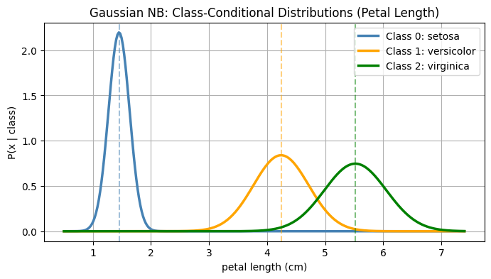
Learned class means for each feature:
  setosa: [4.99 3.45 1.45 0.24]
  versicolor: [5.92 2.77 4.24 1.32]
  virginica: [6.53 2.97 5.52 2.  ]

3. Multinomial Naive Bayes — Text Classification¶

When features are word counts (bag-of-words), the Multinomial NB models each word $w_j$ in class $k$ with a categorical probability:

P(w_j \mid y = k) = \hat{\theta}_{kj} = \frac{\text{count of word } j \text{ in class } k}{\text{total word count in class } k}

(9)

The likelihood of a document $\mathbf{x}$ (word count vector) under class $k$ :

P(\mathbf{x} \mid y = k) = \prod_{j=1}^V \hat{\theta}_{kj}^{x_j}

(10)

Zero-frequency problem: if word $j$ never appears in class $k$ in training, $\hat{\theta}_{kj} = 0$ and the entire likelihood collapses to 0 — even if all other words strongly indicate class $k$ .

Laplace smoothing fixes this by adding a pseudo-count $\alpha$ (default $\alpha = 1$ ):

\hat{\theta}_{kj} = \frac{\text{count}(w_j, k) + \alpha}{\sum_{j'} \text{count}(w_{j'}, k) + \alpha |V|}

(11)

This ensures every word gets a non-zero probability in every class.

Vocabulary representation:

Method	Vector type	sklearn class
Bag of words (count)	Integer counts	`CountVectorizer` + `MultinomialNB`
TF-IDF	Float weights	`TfidfVectorizer` + `ComplementNB`
Word presence (binary)	0/1	`CountVectorizer(binary=True)` + `BernoulliNB`

%matplotlib inline
import numpy as np
import matplotlib.pyplot as plt

class MultinomialNaiveBayes:
    def __init__(self, alpha=1.0):
        self.alpha = alpha

    def fit(self, X, y):
        self.classes_ = np.unique(y)
        n_samples, n_features = X.shape
        self.log_priors_ = {}
        self.log_likelihoods_ = {}
        for k in self.classes_:
            X_k = X[y == k]
            self.log_priors_[k] = np.log(len(X_k) / n_samples)
            word_counts = X_k.sum(axis=0) + self.alpha
            self.log_likelihoods_[k] = np.log(word_counts / word_counts.sum())

    def predict_log_proba(self, X):
        log_proba = np.zeros((len(X), len(self.classes_)))
        for i, k in enumerate(self.classes_):
            log_proba[:, i] = self.log_priors_[k] + X @ self.log_likelihoods_[k]
        return log_proba

    def predict(self, X):
        return self.classes_[np.argmax(self.predict_log_proba(X), axis=1)]


emails = [
    "win a free iPhone today",
    "meeting scheduled at 3pm",
    "earn money working from home",
    "project update attached",
    "free prize winner congratulations",
    "team lunch tomorrow",
    "urgent cash reward offer",
    "report due friday please review",
]
labels = np.array([1, 0, 1, 0, 1, 0, 1, 0])

vocab = sorted(set(w for email in emails for w in email.split()))
word_to_idx = {w: i for i, w in enumerate(vocab)}

X = np.zeros((len(emails), len(vocab)), dtype=float)
for i, email in enumerate(emails):
    for word in email.split():
        X[i, word_to_idx[word]] += 1

mnb = MultinomialNaiveBayes(alpha=1.0)
mnb.fit(X, labels)

test_emails = ["win free cash today", "meeting tomorrow morning"]
X_test = np.zeros((len(test_emails), len(vocab)), dtype=float)
for i, email in enumerate(test_emails):
    for word in email.split():
        if word in word_to_idx:
            X_test[i, word_to_idx[word]] += 1

preds = mnb.predict(X_test)
for email, pred in zip(test_emails, preds):
    print(f'  "{email}" -> {"SPAM" if pred == 1 else "HAM"}')

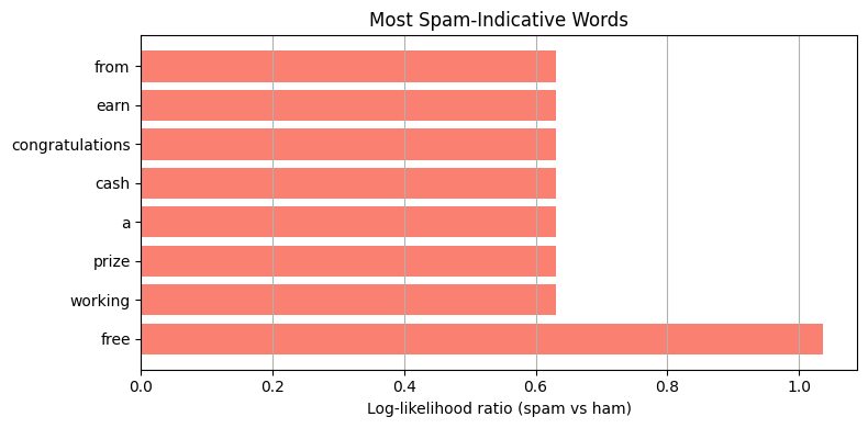
spam_log_ll = mnb.log_likelihoods_[1]
ham_log_ll = mnb.log_likelihoods_[0]
log_ratios = spam_log_ll - ham_log_ll
top_n = 8
top_idx = np.argsort(log_ratios)[-top_n:][::-1]

plt.figure(figsize=(8, 4))
plt.barh([vocab[i] for i in top_idx], log_ratios[top_idx], color='salmon')
plt.xlabel('Log-likelihood ratio (spam vs ham)')
plt.title('Most Spam-Indicative Words')
plt.grid(True, axis='x')
plt.tight_layout()
plt.show()

  "win free cash today" -> SPAM
  "meeting tomorrow morning" -> HAM

4. Laplace Smoothing — The Zero-Frequency Fix¶

Without smoothing, if word ‘prize’ never appears in the ham training emails, $P(\text{prize} \mid \text{ham}) = 0$ and the entire posterior collapses:

P(\text{ham} \mid \text{email}) \propto \ldots \times P(\text{prize} \mid \text{ham}) \times \ldots = 0

(12)

This is wrong — one unseen word should not make the model impossible.

%matplotlib inline
import numpy as np

counts_spam = np.array([10.0, 5.0, 0.0])  # 'free': 10, 'win': 5, 'prize': 0
counts_ham  = np.array([1.0, 0.0, 3.0])   # 'free': 1, 'win': 0, 'prize': 3
test_doc = np.array([1.0, 1.0, 1.0])

alphas = [0.0, 0.01, 0.1, 1.0]
spam_log_posts, ham_log_posts = [], []

for alpha in alphas:
    spam_probs = (counts_spam + alpha) / (counts_spam.sum() + alpha * len(counts_spam))
    ham_probs  = (counts_ham  + alpha) / (counts_ham.sum()  + alpha * len(counts_ham))
    spam_probs = np.maximum(spam_probs, 1e-300)
    ham_probs  = np.maximum(ham_probs,  1e-300)
    spam_log_posts.append(np.sum(test_doc * np.log(spam_probs)))
    ham_log_posts.append(np.sum(test_doc * np.log(ham_probs)))

print(f'{"alpha":>6} | {"log P(spam)":>12} | {"log P(ham)":>10} | Prediction')
print('-' * 50)
for a, sp, hp in zip(alphas, spam_log_posts, ham_log_posts):
    pred = 'SPAM' if sp > hp else 'HAM' if hp > -1e100 else 'UNDEFINED'
    print(f'{a:6.2f} | {sp:12.4f} | {hp:10.4f} | {pred}')

 alpha |  log P(spam) | log P(ham) | Prediction
--------------------------------------------------
  0.00 |    -692.2796 |  -692.4495 | SPAM
  0.01 |      -8.8203 |    -7.6746 | HAM
  0.10 |      -6.5444 |    -5.4517 | HAM
  1.00 |      -4.4815 |    -3.7583 | HAM

5. Naive Bayes with scikit-learn¶

Use sklearn.naive_bayes.MultinomialNB and sklearn.feature_extraction.text.CountVectorizer for a production-grade text pipeline.

%matplotlib inline
import numpy as np
import matplotlib.pyplot as plt
from sklearn.feature_extraction.text import CountVectorizer
from sklearn.naive_bayes import MultinomialNB
from sklearn.model_selection import train_test_split
from sklearn.metrics import accuracy_score, classification_report
from sklearn.pipeline import Pipeline

spam_emails = [
    "win a free iPhone today", "earn money from home fast",
    "urgent cash prize winner", "free gift claim now",
    "limited time offer buy now", "you have been selected winner",
    "get rich quick opportunity", "million dollar lottery prize",
    "free vacation trip winner", "make money online fast",
    "buy cheap medication discount", "click here for free reward",
    "congratulations you won prize", "earn hundreds daily easily",
    "casino bonus free spins",
]
ham_emails = [
    "meeting scheduled for tomorrow", "please review the attached report",
    "team lunch at noon today", "project deadline is next Friday",
    "quarterly review presentation", "budget approval needed soon",
    "conference call at 3pm", "training session next week",
    "office closed on Monday", "interview scheduled for candidate",
    "product roadmap discussion", "sprint retrospective tomorrow",
    "please submit expense report", "client meeting rescheduled",
    "performance review feedback",
]

emails = spam_emails + ham_emails
labels = [1] * len(spam_emails) + [0] * len(ham_emails)

X_train, X_test, y_train, y_test = train_test_split(
    emails, labels, test_size=0.3, random_state=42, stratify=labels
)

pipe = Pipeline([
    ('vect', CountVectorizer()),
    ('clf', MultinomialNB(alpha=1.0)),
])
pipe.fit(X_train, y_train)
y_pred = pipe.predict(X_test)
print('MultinomialNB accuracy:', accuracy_score(y_test, y_pred))
print(classification_report(y_test, y_pred, target_names=['Ham', 'Spam']))

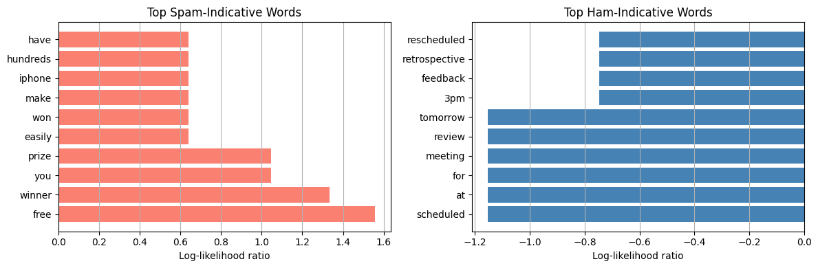
vocab = pipe.named_steps['vect'].get_feature_names_out()
log_probs = pipe.named_steps['clf'].feature_log_prob_
log_ratio = log_probs[1] - log_probs[0]

n = 10
top_spam_idx = np.argsort(log_ratio)[-n:][::-1]
top_ham_idx = np.argsort(log_ratio)[:n]

fig, axes = plt.subplots(1, 2, figsize=(12, 4))
axes[0].barh([vocab[i] for i in top_spam_idx], log_ratio[top_spam_idx], color='salmon')
axes[0].set_title('Top Spam-Indicative Words')
axes[0].set_xlabel('Log-likelihood ratio')
axes[0].grid(True, axis='x')

axes[1].barh([vocab[i] for i in top_ham_idx], log_ratio[top_ham_idx], color='steelblue')
axes[1].set_title('Top Ham-Indicative Words')
axes[1].set_xlabel('Log-likelihood ratio')
axes[1].grid(True, axis='x')

plt.tight_layout()
plt.show()

MultinomialNB accuracy: 0.6666666666666666
              precision    recall  f1-score   support

         Ham       1.00      0.40      0.57         5
        Spam       0.57      1.00      0.73         4

    accuracy                           0.67         9
   macro avg       0.79      0.70      0.65         9
weighted avg       0.81      0.67      0.64         9

6. Generative vs Discriminative — Naive Bayes vs Logistic Regression¶

Dimension	Naive Bayes	Logistic Regression
Approach	Generative: models $P(\mathbf{x}	y)$
Training	Closed-form MLE (one pass)	Iterative gradient descent
Speed	Very fast	Slower
Data efficiency	Works well with small data	Needs more data to beat NB
Feature correlation	Independence assumption hurts	Handles correlated features
Probabilities	Often miscalibrated	Better calibrated
Text data	Excellent	Good but slower

Rule of thumb: use NB for small data / text; use LR for larger tabular data where calibration matters.

7. Try It in the Browser¶

A minimal Gaussian NB in pure Python — adjust training data to see how posteriors change.

import math

def gaussian_pdf(x, mu, sigma2):
    return (1.0 / math.sqrt(2 * math.pi * sigma2)) * math.exp(-0.5 * (x - mu)**2 / sigma2)

# Feature = height_cm, classes = {0: short, 1: tall}
data = [
    (160, 0), (165, 0), (155, 0), (170, 0), (163, 0),
    (185, 1), (180, 1), (190, 1), (175, 1), (183, 1),
]

classes = [0, 1]
params = {}
for k in classes:
    vals = [x for x, y in data if y == k]
    mu = sum(vals) / len(vals)
    var = sum((v - mu)**2 for v in vals) / len(vals) + 1e-6
    prior = len(vals) / len(data)
    params[k] = {'mu': mu, 'var': var, 'prior': prior}

x_new = 172
log_posts = {}
for k in classes:
    ll = math.log(gaussian_pdf(x_new, params[k]['mu'], params[k]['var']) + 1e-300)
    log_posts[k] = math.log(params[k]['prior']) + ll

print(f'Predicting for x = {x_new} cm')
print(f'  Class 0 (short): log-posterior = {log_posts[0]:.4f}')
print(f'  Class 1 (tall):  log-posterior = {log_posts[1]:.4f}')
pred = max(log_posts, key=log_posts.get)
print(f'  Prediction: {"tall" if pred == 1 else "short"}')

Knowledge Check¶

Why is Naive Bayes called "naive"?¶

Because it assumes features are conditionally independent given the classCorrect. That simplifying assumption is what gives the method its name.

Because it cannot produce probabilitiesNaive Bayes is explicitly probabilistic.

Because it uses no data at allIt still learns from observed data.

Because it is always inaccurateDespite the assumption, it can work very well in some domains.

In what kind of setting can Naive Bayes perform surprisingly well?¶

Only on time series forecasting with continuous outputsThat is not a standard Naive Bayes use case.

On high-dimensional problems such as text classificationCorrect. Naive Bayes is often effective for text and sparse-feature tasks.

Only when all classes are already perfectly separatedIt is not restricted to perfect separation.

Only when no probabilities are neededNaive Bayes naturally provides probability-based outputs.

What does Laplace smoothing fix in Multinomial Naive Bayes?¶

It prevents overfitting by penalising large weightsThat is regularisation, not Laplace smoothing.

It prevents zero likelihoods from a word unseen in a training classCorrect. Adding a pseudo-count ensures every word has a non-zero probability.

It normalises the feature vectors to unit lengthThat is a different operation.

It increases the size of the training vocabularySmoothing adjusts probability estimates, not vocabulary size.

When computing the MAP decision rule, why is the evidence P(x) ignored?¶

Because P(x) is always equal to 1P(x) is a valid probability sum, not necessarily 1.

Because P(x) is the same constant across all classes and does not affect which class has the highest posteriorCorrect. Since we are taking argmax over classes, a shared denominator cancels.

Because P(x) is always zero for unseen dataP(x) is generally non-zero; it just drops from the argmax.

Because computing it requires access to all possible classesP(x) can be computed but it cancels in argmax.

Exercises¶

Exercise 1 — Gaussian NB on Wine Dataset¶

Load the wine dataset from sklearn. Fit your GaussianNaiveBayes class and compute test accuracy. Compare to sklearn’s GaussianNB. Do the results match?

%matplotlib inline
# Exercise 1: Gaussian NB on wine dataset
# Your code here

Exercise 2 — Smoothing Strength¶

Using the spam pipeline above, sweep alpha over [0.001, 0.01, 0.1, 1.0, 10.0] and plot test accuracy vs alpha. Does more smoothing always help?

%matplotlib inline
# Exercise 2: Laplace smoothing sweep
# Your code here

Common Pitfalls¶

What’s Next?¶

Both logistic regression and Naive Bayes assume the training data is representative — but real business datasets are often severely class-imbalanced (e.g., 1 % fraud, 99 % legitimate). In class_imbalance.ipynb we tackle calibration, SMOTE, class weights, and how to evaluate imbalanced classifiers correctly.

Coming up:

Calibration & Class Imbalance — reliability diagrams, SMOTE, cost-sensitive learning
Classification Metrics — precision, recall, F1, AUC-ROC, AUC-PR in depth
Lab — Churn Prediction end-to-end pipeline