Calibration & Class Imbalance¶

Learning objectives

By the end of this notebook you will be able to:

Explain why accuracy is misleading on imbalanced datasets.
Demonstrate the accuracy illusion with a concrete example.
Apply class weighting to re-balance the loss function.
Use SMOTE to oversample the minority class synthetically.
Understand what probability calibration means and why it matters.
Build a reliability diagram and interpret it.
Apply Platt scaling and isotonic regression to calibrate a classifier.
Choose the right strategy for a given imbalance scenario.

Business hook — The 95 % lie¶

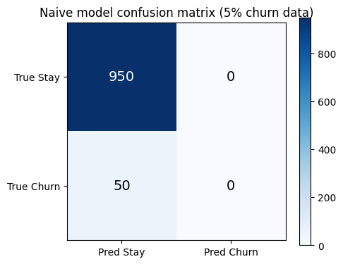
A bank’s fraud detection model achieves 95 % accuracy. The data science team is proud. Then the risk team asks: “How many frauds did you catch?” Answer: zero. Every single transaction was predicted as legitimate — because 95 % of transactions are legitimate.

This is the accuracy illusion — the most common trap in production classification. The model learned to exploit class imbalance rather than detect the minority class.

1. The Accuracy Illusion¶

%matplotlib inline
import numpy as np
import matplotlib.pyplot as plt
from sklearn.metrics import accuracy_score, classification_report, confusion_matrix

# Simulate 5% churn rate (imbalanced dataset)
np.random.seed(42)
n = 1000
y_true = np.array([0]*950 + [1]*50)

# Naive model: always predict majority class
y_naive = np.zeros(n, dtype=int)

print('=== Naive model (always predict 0) ===')
print(f'Accuracy: {accuracy_score(y_true, y_naive):.3f}')
print(classification_report(y_true, y_naive, target_names=['Stay', 'Churn'], zero_division=0))

# Visualise the confusion matrix
cm = confusion_matrix(y_true, y_naive)
fig, ax = plt.subplots(figsize=(5, 4))
im = ax.imshow(cm, cmap='Blues')
for i in range(2):
    for j in range(2):
        ax.text(j, i, str(cm[i, j]), ha='center', va='center', fontsize=14,
                color='white' if cm[i, j] > cm.max()/2 else 'black')
ax.set_xticks([0, 1]); ax.set_yticks([0, 1])
ax.set_xticklabels(['Pred Stay', 'Pred Churn'])
ax.set_yticklabels(['True Stay', 'True Churn'])
ax.set_title('Naive model confusion matrix (5% churn data)')
plt.colorbar(im)
plt.tight_layout()
plt.show()

=== Naive model (always predict 0) ===
Accuracy: 0.950
              precision    recall  f1-score   support

        Stay       0.95      1.00      0.97       950
       Churn       0.00      0.00      0.00        50

    accuracy                           0.95      1000
   macro avg       0.47      0.50      0.49      1000
weighted avg       0.90      0.95      0.93      1000

2. Class Weights — Re-balancing the Loss¶

The simplest fix is to weight the loss differently for majority vs minority class samples:

J_{\text{weighted}} = -\frac{1}{n} \sum_{i=1}^n w_{y^{(i)}} \left[ y^{(i)} \log \hat{y}^{(i)} + (1-y^{(i)}) \log(1-\hat{y}^{(i)}) \right]

(1)

With class_weight='balanced', sklearn sets:

w_k = \frac{n}{K \cdot n_k}

(2)

where $n_k$ is the count of class $k$ and $K$ is the number of classes. Rare class samples count more in the gradient update — the model can no longer ignore them.

When to use class weights:

You want to keep all training data (no information discarded).
The imbalance is moderate (< 100:1).
You are using a model that supports class_weight (most sklearn classifiers do).

%matplotlib inline
import numpy as np
import matplotlib.pyplot as plt
from sklearn.datasets import make_classification
from sklearn.linear_model import LogisticRegression
from sklearn.model_selection import train_test_split
from sklearn.metrics import f1_score, recall_score, precision_score, roc_auc_score

# Imbalanced dataset: 5% positive class
X, y = make_classification(
    n_samples=2000, n_features=10, n_informative=5,
    weights=[0.95, 0.05], random_state=42, flip_y=0.01
)
X_train, X_test, y_train, y_test = train_test_split(X, y, test_size=0.2, random_state=42, stratify=y)

results = {}
for label, cw in [('No weight', None), ('class_weight=balanced', 'balanced')]:
    m = LogisticRegression(class_weight=cw, max_iter=1000, random_state=42)
    m.fit(X_train, y_train)
    y_pred = m.predict(X_test)
    results[label] = {
        'F1': f1_score(y_test, y_pred, zero_division=0),
        'Recall': recall_score(y_test, y_pred, zero_division=0),
        'Precision': precision_score(y_test, y_pred, zero_division=0),
        'AUC': roc_auc_score(y_test, m.predict_proba(X_test)[:, 1]),
    }

metrics = ['F1', 'Recall', 'Precision', 'AUC']
x = np.arange(len(metrics))
width = 0.35
fig, ax = plt.subplots(figsize=(9, 4))
for i, (label, vals) in enumerate(results.items()):
    ax.bar(x + i*width - width/2, [vals[m] for m in metrics], width, label=label)
ax.set_xticks(x); ax.set_xticklabels(metrics)
ax.set_ylim(0, 1.1)
ax.set_ylabel('Score')
ax.set_title('Effect of Class Weighting on Imbalanced Dataset')
ax.legend()
ax.grid(True, axis='y', alpha=0.3)
plt.tight_layout()
plt.show()

for label, vals in results.items():
    print(f'{label}: F1={vals["F1"]:.3f}, Recall={vals["Recall"]:.3f}, Precision={vals["Precision"]:.3f}, AUC={vals["AUC"]:.3f}')

/Volumes/MacSSD/01_Projects/Chandravesh-ML-Research/projects/jupyter-books/.venv/lib/python3.10/site-packages/sklearn/linear_model/_linear_loss.py:200: RuntimeWarning: divide by zero encountered in matmul
  raw_prediction = X @ weights + intercept
/Volumes/MacSSD/01_Projects/Chandravesh-ML-Research/projects/jupyter-books/.venv/lib/python3.10/site-packages/sklearn/linear_model/_linear_loss.py:200: RuntimeWarning: overflow encountered in matmul
  raw_prediction = X @ weights + intercept
/Volumes/MacSSD/01_Projects/Chandravesh-ML-Research/projects/jupyter-books/.venv/lib/python3.10/site-packages/sklearn/linear_model/_linear_loss.py:200: RuntimeWarning: invalid value encountered in matmul
  raw_prediction = X @ weights + intercept
/Volumes/MacSSD/01_Projects/Chandravesh-ML-Research/projects/jupyter-books/.venv/lib/python3.10/site-packages/sklearn/linear_model/_linear_loss.py:330: RuntimeWarning: divide by zero encountered in matmul
  grad[:n_features] = X.T @ grad_pointwise + l2_reg_strength * weights
/Volumes/MacSSD/01_Projects/Chandravesh-ML-Research/projects/jupyter-books/.venv/lib/python3.10/site-packages/sklearn/linear_model/_linear_loss.py:330: RuntimeWarning: overflow encountered in matmul
  grad[:n_features] = X.T @ grad_pointwise + l2_reg_strength * weights
/Volumes/MacSSD/01_Projects/Chandravesh-ML-Research/projects/jupyter-books/.venv/lib/python3.10/site-packages/sklearn/linear_model/_linear_loss.py:330: RuntimeWarning: invalid value encountered in matmul
  grad[:n_features] = X.T @ grad_pointwise + l2_reg_strength * weights
/Volumes/MacSSD/01_Projects/Chandravesh-ML-Research/projects/jupyter-books/.venv/lib/python3.10/site-packages/sklearn/utils/extmath.py:203: RuntimeWarning: divide by zero encountered in matmul
  ret = a @ b
/Volumes/MacSSD/01_Projects/Chandravesh-ML-Research/projects/jupyter-books/.venv/lib/python3.10/site-packages/sklearn/utils/extmath.py:203: RuntimeWarning: overflow encountered in matmul
  ret = a @ b
/Volumes/MacSSD/01_Projects/Chandravesh-ML-Research/projects/jupyter-books/.venv/lib/python3.10/site-packages/sklearn/utils/extmath.py:203: RuntimeWarning: invalid value encountered in matmul
  ret = a @ b
/Volumes/MacSSD/01_Projects/Chandravesh-ML-Research/projects/jupyter-books/.venv/lib/python3.10/site-packages/sklearn/utils/extmath.py:203: RuntimeWarning: divide by zero encountered in matmul
  ret = a @ b
/Volumes/MacSSD/01_Projects/Chandravesh-ML-Research/projects/jupyter-books/.venv/lib/python3.10/site-packages/sklearn/utils/extmath.py:203: RuntimeWarning: overflow encountered in matmul
  ret = a @ b
/Volumes/MacSSD/01_Projects/Chandravesh-ML-Research/projects/jupyter-books/.venv/lib/python3.10/site-packages/sklearn/utils/extmath.py:203: RuntimeWarning: invalid value encountered in matmul
  ret = a @ b
/Volumes/MacSSD/01_Projects/Chandravesh-ML-Research/projects/jupyter-books/.venv/lib/python3.10/site-packages/sklearn/linear_model/_linear_loss.py:200: RuntimeWarning: divide by zero encountered in matmul
  raw_prediction = X @ weights + intercept
/Volumes/MacSSD/01_Projects/Chandravesh-ML-Research/projects/jupyter-books/.venv/lib/python3.10/site-packages/sklearn/linear_model/_linear_loss.py:200: RuntimeWarning: overflow encountered in matmul
  raw_prediction = X @ weights + intercept
/Volumes/MacSSD/01_Projects/Chandravesh-ML-Research/projects/jupyter-books/.venv/lib/python3.10/site-packages/sklearn/linear_model/_linear_loss.py:200: RuntimeWarning: invalid value encountered in matmul
  raw_prediction = X @ weights + intercept
/Volumes/MacSSD/01_Projects/Chandravesh-ML-Research/projects/jupyter-books/.venv/lib/python3.10/site-packages/sklearn/linear_model/_linear_loss.py:330: RuntimeWarning: divide by zero encountered in matmul
  grad[:n_features] = X.T @ grad_pointwise + l2_reg_strength * weights
/Volumes/MacSSD/01_Projects/Chandravesh-ML-Research/projects/jupyter-books/.venv/lib/python3.10/site-packages/sklearn/linear_model/_linear_loss.py:330: RuntimeWarning: overflow encountered in matmul
  grad[:n_features] = X.T @ grad_pointwise + l2_reg_strength * weights
/Volumes/MacSSD/01_Projects/Chandravesh-ML-Research/projects/jupyter-books/.venv/lib/python3.10/site-packages/sklearn/linear_model/_linear_loss.py:330: RuntimeWarning: invalid value encountered in matmul
  grad[:n_features] = X.T @ grad_pointwise + l2_reg_strength * weights
/Volumes/MacSSD/01_Projects/Chandravesh-ML-Research/projects/jupyter-books/.venv/lib/python3.10/site-packages/sklearn/utils/extmath.py:203: RuntimeWarning: divide by zero encountered in matmul
  ret = a @ b
/Volumes/MacSSD/01_Projects/Chandravesh-ML-Research/projects/jupyter-books/.venv/lib/python3.10/site-packages/sklearn/utils/extmath.py:203: RuntimeWarning: overflow encountered in matmul
  ret = a @ b
/Volumes/MacSSD/01_Projects/Chandravesh-ML-Research/projects/jupyter-books/.venv/lib/python3.10/site-packages/sklearn/utils/extmath.py:203: RuntimeWarning: invalid value encountered in matmul
  ret = a @ b
/Volumes/MacSSD/01_Projects/Chandravesh-ML-Research/projects/jupyter-books/.venv/lib/python3.10/site-packages/sklearn/utils/extmath.py:203: RuntimeWarning: divide by zero encountered in matmul
  ret = a @ b
/Volumes/MacSSD/01_Projects/Chandravesh-ML-Research/projects/jupyter-books/.venv/lib/python3.10/site-packages/sklearn/utils/extmath.py:203: RuntimeWarning: overflow encountered in matmul
  ret = a @ b
/Volumes/MacSSD/01_Projects/Chandravesh-ML-Research/projects/jupyter-books/.venv/lib/python3.10/site-packages/sklearn/utils/extmath.py:203: RuntimeWarning: invalid value encountered in matmul
  ret = a @ b

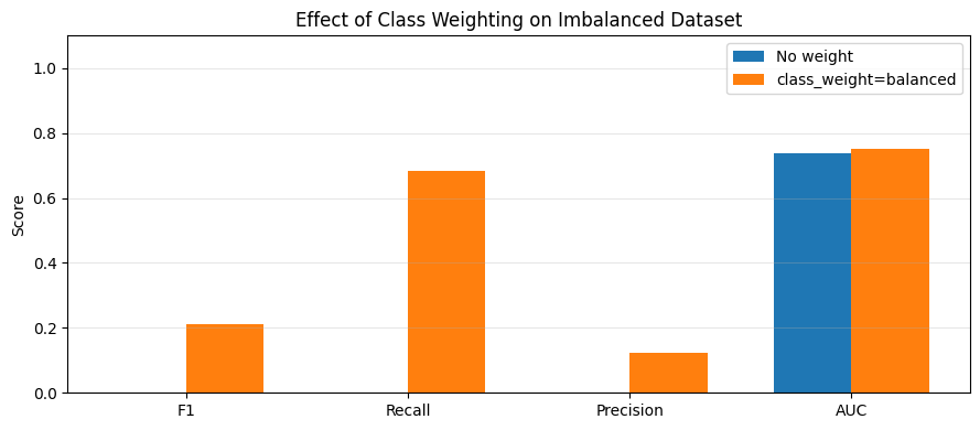
No weight: F1=0.000, Recall=0.000, Precision=0.000, AUC=0.737
class_weight=balanced: F1=0.210, Recall=0.682, Precision=0.124, AUC=0.753

3. SMOTE — Synthetic Minority Over-Sampling¶

SMOTE (Chawla et al., 2002) creates synthetic minority class samples by interpolating between existing minority samples and their k nearest neighbours:

\mathbf{x}_{\text{new}} = \mathbf{x}_i + \lambda \cdot (\mathbf{x}_{\text{nn}} - \mathbf{x}_i), \quad \lambda \sim \text{Uniform}(0, 1)

(3)

This avoids the exact duplication problem of naive random oversampling (which just copies existing minority examples).

When to use SMOTE vs class weights:

Strategy	Best for	Risk
Class weights	Moderate imbalance, any model	May not handle extreme imbalance
Random oversampling	Quick fix	Overfits to existing minority examples
SMOTE	Tree models, extreme imbalance	Can create noise in overlapping regions
Random undersampling	Very large datasets	Throws away majority class information

Important: always apply resampling only to the training set — never to validation or test.

%matplotlib inline
import numpy as np
import matplotlib.pyplot as plt
from sklearn.datasets import make_classification
from sklearn.model_selection import train_test_split
from sklearn.metrics import f1_score

# SMOTE from scratch (simplified 1D illustration)
def simple_smote(X_minority, n_synthetic, k=3, random_state=42):
    np.random.seed(random_state)
    synthetic = []
    for _ in range(n_synthetic):
        i = np.random.randint(len(X_minority))
        xi = X_minority[i]
        # Find k nearest neighbours
        dists = np.linalg.norm(X_minority - xi, axis=1)
        dists[i] = np.inf
        nn_idx = np.argsort(dists)[:k]
        nn = X_minority[np.random.choice(nn_idx)]
        lam = np.random.uniform(0, 1)
        synthetic.append(xi + lam * (nn - xi))
    return np.array(synthetic)

# Generate 2D imbalanced data for visualisation
X, y = make_classification(
    n_samples=300, n_features=2, n_redundant=0, n_informative=2,
    weights=[0.9, 0.1], random_state=42, class_sep=1.5
)

X_min = X[y == 1]
n_synthetic = len(X[y == 0]) - len(X_min)  # balance the classes
X_synthetic = simple_smote(X_min, n_synthetic)

fig, axes = plt.subplots(1, 2, figsize=(12, 5))

axes[0].scatter(X[y==0, 0], X[y==0, 1], c='steelblue', alpha=0.4, label='Majority (0)', s=20)
axes[0].scatter(X[y==1, 0], X[y==1, 1], c='red', alpha=0.8, label='Minority (1)', s=50)
axes[0].set_title(f'Before SMOTE: {sum(y==0)} vs {sum(y==1)} samples')
axes[0].legend()
axes[0].grid(True)

axes[1].scatter(X[y==0, 0], X[y==0, 1], c='steelblue', alpha=0.4, label='Majority (0)', s=20)
axes[1].scatter(X[y==1, 0], X[y==1, 1], c='red', alpha=0.8, label='Original minority', s=50)
axes[1].scatter(X_synthetic[:, 0], X_synthetic[:, 1], c='orange', alpha=0.6, label='SMOTE synthetic', s=20, marker='+')
axes[1].set_title(f'After SMOTE: balanced {sum(y==0)} vs {sum(y==1)+len(X_synthetic)}')
axes[1].legend()
axes[1].grid(True)

plt.suptitle('SMOTE: Synthetic Minority Over-Sampling', fontsize=12)
plt.tight_layout()
plt.show()

# Compare with imbalanced-learn if available
try:
    from imblearn.over_sampling import SMOTE
    from sklearn.linear_model import LogisticRegression
    X_train, X_test, y_train, y_test = train_test_split(X, y, test_size=0.2, random_state=42, stratify=y)
    sm = SMOTE(random_state=42)
    X_res, y_res = sm.fit_resample(X_train, y_train)
    m1 = LogisticRegression(max_iter=1000).fit(X_train, y_train)
    m2 = LogisticRegression(max_iter=1000).fit(X_res, y_res)
    print(f'F1 without SMOTE: {f1_score(y_test, m1.predict(X_test)):.3f}')
    print(f'F1 with SMOTE:    {f1_score(y_test, m2.predict(X_test)):.3f}')
except ImportError:
    print('imbalanced-learn not installed. Install with: pip install imbalanced-learn')
    print('SMOTE visualisation complete.')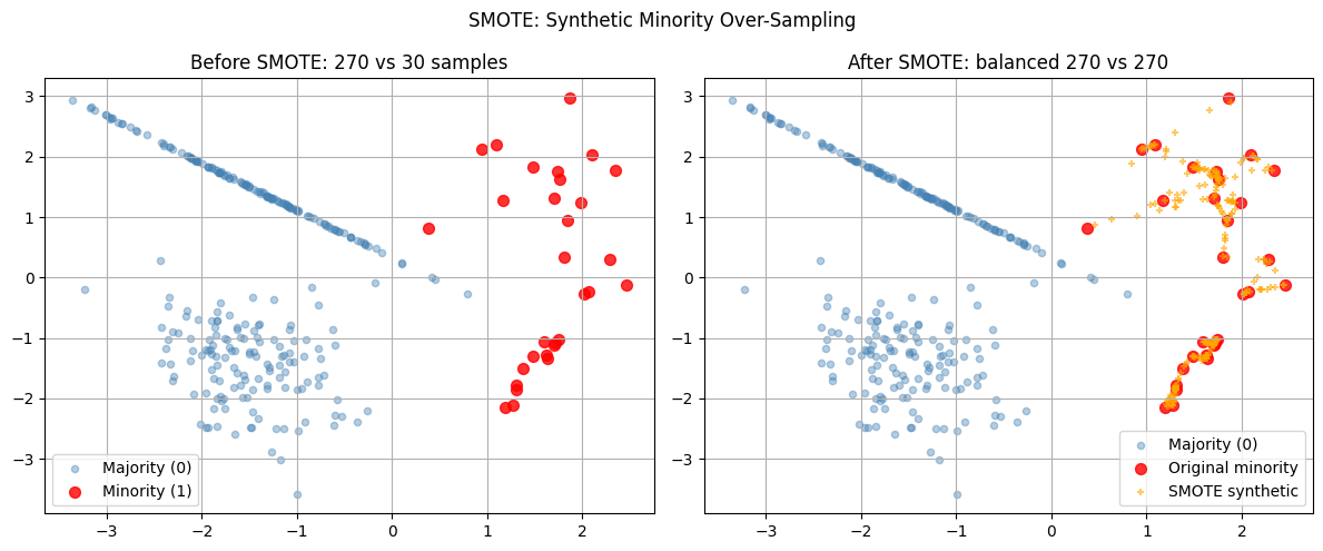

imbalanced-learn not installed. Install with: pip install imbalanced-learn
SMOTE visualisation complete.

4. Probability Calibration¶

A calibrated classifier is one where the predicted probability $\hat{p}$ accurately reflects the empirical frequency. If a calibrated model says “80 % churn probability”, then roughly 80 of every 100 such predictions should actually churn.

Why calibration matters for business:

Setting decision thresholds (“call customer if churn prob > 0.7”)
Expected value calculations ( $EV = p \times \text{revenue} - \text{cost}$ )
Stacking models: miscalibrated outputs feed bad signals to the next layer

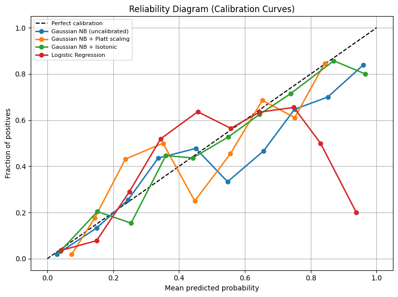
Reliability diagram (calibration curve): plot mean predicted probability vs empirical frequency per bin. A perfectly calibrated model follows the diagonal.

Model type	Typical calibration issue
Naive Bayes	Overconfident — pushes probs to 0/1
Logistic Regression	Well-calibrated by design
Random Forest	Under-confident — probs cluster near 0.5
Gradient Boosting	Under-confident near extremes
SVM	Poor — scores not probabilities

Calibration methods:

Platt scaling: fit a logistic regression on $\hat{p}$ values (sigmoid transform)
Isotonic regression: fit a monotonic step function — more flexible, needs more data

%matplotlib inline
import numpy as np
import matplotlib.pyplot as plt
from sklearn.datasets import make_classification
from sklearn.model_selection import train_test_split
from sklearn.naive_bayes import GaussianNB
from sklearn.linear_model import LogisticRegression
from sklearn.calibration import calibration_curve, CalibratedClassifierCV

X, y = make_classification(
    n_samples=2000, n_features=10, n_informative=5,
    weights=[0.7, 0.3], random_state=42
)
X_train, X_test, y_train, y_test = train_test_split(X, y, test_size=0.3, random_state=42)

models = {
    'Gaussian NB (uncalibrated)': GaussianNB(),
    'Gaussian NB + Platt scaling': CalibratedClassifierCV(GaussianNB(), cv=5, method='sigmoid'),
    'Gaussian NB + Isotonic':      CalibratedClassifierCV(GaussianNB(), cv=5, method='isotonic'),
    'Logistic Regression':         LogisticRegression(max_iter=1000, random_state=42),
}

plt.figure(figsize=(8, 6))
plt.plot([0, 1], [0, 1], 'k--', label='Perfect calibration')

for name, m in models.items():
    m.fit(X_train, y_train)
    prob_pos = m.predict_proba(X_test)[:, 1]
    fraction_of_positives, mean_predicted_value = calibration_curve(y_test, prob_pos, n_bins=10)
    plt.plot(mean_predicted_value, fraction_of_positives, marker='o', linewidth=2, label=name)

plt.xlabel('Mean predicted probability')
plt.ylabel('Fraction of positives')
plt.title('Reliability Diagram (Calibration Curves)')
plt.legend(loc='upper left', fontsize=8)
plt.grid(True)
plt.tight_layout()
plt.show()

/Volumes/MacSSD/01_Projects/Chandravesh-ML-Research/projects/jupyter-books/.venv/lib/python3.10/site-packages/sklearn/linear_model/_linear_loss.py:200: RuntimeWarning: divide by zero encountered in matmul
  raw_prediction = X @ weights + intercept
/Volumes/MacSSD/01_Projects/Chandravesh-ML-Research/projects/jupyter-books/.venv/lib/python3.10/site-packages/sklearn/linear_model/_linear_loss.py:200: RuntimeWarning: overflow encountered in matmul
  raw_prediction = X @ weights + intercept
/Volumes/MacSSD/01_Projects/Chandravesh-ML-Research/projects/jupyter-books/.venv/lib/python3.10/site-packages/sklearn/linear_model/_linear_loss.py:200: RuntimeWarning: invalid value encountered in matmul
  raw_prediction = X @ weights + intercept
/Volumes/MacSSD/01_Projects/Chandravesh-ML-Research/projects/jupyter-books/.venv/lib/python3.10/site-packages/sklearn/linear_model/_linear_loss.py:330: RuntimeWarning: divide by zero encountered in matmul
  grad[:n_features] = X.T @ grad_pointwise + l2_reg_strength * weights
/Volumes/MacSSD/01_Projects/Chandravesh-ML-Research/projects/jupyter-books/.venv/lib/python3.10/site-packages/sklearn/linear_model/_linear_loss.py:330: RuntimeWarning: overflow encountered in matmul
  grad[:n_features] = X.T @ grad_pointwise + l2_reg_strength * weights
/Volumes/MacSSD/01_Projects/Chandravesh-ML-Research/projects/jupyter-books/.venv/lib/python3.10/site-packages/sklearn/linear_model/_linear_loss.py:330: RuntimeWarning: invalid value encountered in matmul
  grad[:n_features] = X.T @ grad_pointwise + l2_reg_strength * weights
/Volumes/MacSSD/01_Projects/Chandravesh-ML-Research/projects/jupyter-books/.venv/lib/python3.10/site-packages/sklearn/utils/extmath.py:203: RuntimeWarning: divide by zero encountered in matmul
  ret = a @ b
/Volumes/MacSSD/01_Projects/Chandravesh-ML-Research/projects/jupyter-books/.venv/lib/python3.10/site-packages/sklearn/utils/extmath.py:203: RuntimeWarning: overflow encountered in matmul
  ret = a @ b
/Volumes/MacSSD/01_Projects/Chandravesh-ML-Research/projects/jupyter-books/.venv/lib/python3.10/site-packages/sklearn/utils/extmath.py:203: RuntimeWarning: invalid value encountered in matmul
  ret = a @ b

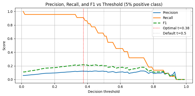
5. Threshold Selection under Imbalance¶

The default 0.5 threshold is derived assuming balanced classes. On imbalanced data, the optimal threshold is typically lower for the positive class (to increase recall).

Strategy: sweep the threshold and optimise for the business metric (F1, expected value, or a precision-recall tradeoff).

%matplotlib inline
import numpy as np
import matplotlib.pyplot as plt
from sklearn.datasets import make_classification
from sklearn.linear_model import LogisticRegression
from sklearn.model_selection import train_test_split
from sklearn.metrics import precision_score, recall_score, f1_score

X, y = make_classification(
    n_samples=2000, n_features=10, n_informative=5,
    weights=[0.95, 0.05], random_state=42
)
X_train, X_test, y_train, y_test = train_test_split(X, y, test_size=0.2, random_state=42, stratify=y)

m = LogisticRegression(class_weight='balanced', max_iter=1000, random_state=42)
m.fit(X_train, y_train)
probs = m.predict_proba(X_test)[:, 1]

thresholds = np.linspace(0.01, 0.99, 100)
precisions, recalls, f1s = [], [], []
for t in thresholds:
    y_pred_t = (probs >= t).astype(int)
    precisions.append(precision_score(y_test, y_pred_t, zero_division=0))
    recalls.append(recall_score(y_test, y_pred_t, zero_division=0))
    f1s.append(f1_score(y_test, y_pred_t, zero_division=0))

best_t = thresholds[np.argmax(f1s)]
print(f'Optimal threshold for max F1: {best_t:.3f}')
print(f'At threshold 0.5: F1={f1_score(y_test, (probs>=0.5).astype(int)):.3f}')
print(f'At optimal threshold {best_t:.3f}: F1={max(f1s):.3f}')

plt.figure(figsize=(8, 4))
plt.plot(thresholds, precisions, label='Precision', linewidth=2)
plt.plot(thresholds, recalls, label='Recall', linewidth=2)
plt.plot(thresholds, f1s, label='F1', linewidth=2.5, linestyle='--')
plt.axvline(best_t, color='red', linestyle=':', label=f'Optimal t={best_t:.2f}')
plt.axvline(0.5, color='gray', linestyle=':', alpha=0.5, label='Default t=0.5')
plt.xlabel('Decision threshold')
plt.ylabel('Score')
plt.title('Precision, Recall, and F1 vs Threshold (5% positive class)')
plt.legend()
plt.grid(True)
plt.tight_layout()
plt.show()

/Volumes/MacSSD/01_Projects/Chandravesh-ML-Research/projects/jupyter-books/.venv/lib/python3.10/site-packages/sklearn/linear_model/_linear_loss.py:200: RuntimeWarning: divide by zero encountered in matmul
  raw_prediction = X @ weights + intercept
/Volumes/MacSSD/01_Projects/Chandravesh-ML-Research/projects/jupyter-books/.venv/lib/python3.10/site-packages/sklearn/linear_model/_linear_loss.py:200: RuntimeWarning: overflow encountered in matmul
  raw_prediction = X @ weights + intercept
/Volumes/MacSSD/01_Projects/Chandravesh-ML-Research/projects/jupyter-books/.venv/lib/python3.10/site-packages/sklearn/linear_model/_linear_loss.py:200: RuntimeWarning: invalid value encountered in matmul
  raw_prediction = X @ weights + intercept
/Volumes/MacSSD/01_Projects/Chandravesh-ML-Research/projects/jupyter-books/.venv/lib/python3.10/site-packages/sklearn/linear_model/_linear_loss.py:330: RuntimeWarning: divide by zero encountered in matmul
  grad[:n_features] = X.T @ grad_pointwise + l2_reg_strength * weights
/Volumes/MacSSD/01_Projects/Chandravesh-ML-Research/projects/jupyter-books/.venv/lib/python3.10/site-packages/sklearn/linear_model/_linear_loss.py:330: RuntimeWarning: overflow encountered in matmul
  grad[:n_features] = X.T @ grad_pointwise + l2_reg_strength * weights
/Volumes/MacSSD/01_Projects/Chandravesh-ML-Research/projects/jupyter-books/.venv/lib/python3.10/site-packages/sklearn/linear_model/_linear_loss.py:330: RuntimeWarning: invalid value encountered in matmul
  grad[:n_features] = X.T @ grad_pointwise + l2_reg_strength * weights
/Volumes/MacSSD/01_Projects/Chandravesh-ML-Research/projects/jupyter-books/.venv/lib/python3.10/site-packages/sklearn/utils/extmath.py:203: RuntimeWarning: divide by zero encountered in matmul
  ret = a @ b
/Volumes/MacSSD/01_Projects/Chandravesh-ML-Research/projects/jupyter-books/.venv/lib/python3.10/site-packages/sklearn/utils/extmath.py:203: RuntimeWarning: overflow encountered in matmul
  ret = a @ b
/Volumes/MacSSD/01_Projects/Chandravesh-ML-Research/projects/jupyter-books/.venv/lib/python3.10/site-packages/sklearn/utils/extmath.py:203: RuntimeWarning: invalid value encountered in matmul
  ret = a @ b

Optimal threshold for max F1: 0.376
At threshold 0.5: F1=0.210
At optimal threshold 0.376: F1=0.216

6. Try It in the Browser¶

See the accuracy illusion in pure Python — then observe how class weights change the outcome.

import math
import random

random.seed(42)

def sigmoid(z):
    return 1.0 / (1.0 + math.exp(-max(-500, min(500, z))))

# 5% positive class
n_neg, n_pos = 950, 50
X = [(random.gauss(-1, 1), 0) for _ in range(n_neg)] + [(random.gauss(1, 1), 1) for _ in range(n_pos)]
random.shuffle(X)
xs, ys = [x for x, y in X], [y for x, y in X]

def train_lr(xs, ys, w_pos=1.0, lr=0.5, epochs=200):
    w, b = 0.0, 0.0
    for _ in range(epochs):
        for xi, yi in zip(xs, ys):
            weight = w_pos if yi == 1 else 1.0
            yhat = sigmoid(w * xi + b)
            err = yhat - yi
            w -= lr * weight * err * xi / len(xs)
            b -= lr * weight * err / len(xs)
    return w, b

def evaluate(w, b, xs, ys, threshold=0.5):
    preds = [1 if sigmoid(w*xi + b) >= threshold else 0 for xi in xs]
    acc = sum(p == y for p, y in zip(preds, ys)) / len(ys)
    tp = sum(p == 1 and y == 1 for p, y in zip(preds, ys))
    fp = sum(p == 1 and y == 0 for p, y in zip(preds, ys))
    fn = sum(p == 0 and y == 1 for p, y in zip(preds, ys))
    prec = tp / (tp + fp) if (tp + fp) > 0 else 0.0
    rec = tp / (tp + fn) if (tp + fn) > 0 else 0.0
    f1 = 2 * prec * rec / (prec + rec) if (prec + rec) > 0 else 0.0
    return acc, prec, rec, f1

# Without class weights
w1, b1 = train_lr(xs, ys, w_pos=1.0)
acc1, prec1, rec1, f1_1 = evaluate(w1, b1, xs, ys)
print('Without class weights:')
print(f'  Accuracy={acc1:.2%}, Precision={prec1:.2%}, Recall={rec1:.2%}, F1={f1_1:.2%}')

# With class weights (19x for minority)
w2, b2 = train_lr(xs, ys, w_pos=19.0)
acc2, prec2, rec2, f1_2 = evaluate(w2, b2, xs, ys)
print('With class weights (w_pos=19):')
print(f'  Accuracy={acc2:.2%}, Precision={prec2:.2%}, Recall={rec2:.2%}, F1={f1_2:.2%}')

Knowledge Check¶

Why can accuracy be misleading on a highly imbalanced dataset?¶

Because a model can predict the majority class always and still appear strongCorrect. High accuracy can hide poor detection of the minority class.

Because accuracy becomes undefined mathematicallyAccuracy remains defined, but it may be uninformative.

Because imbalance removes the target labelsThe labels still exist.

Because all minority examples are automatically misclassifiedThat is possible but not automatic.

What is the purpose of probability calibration?¶

To change the labels in the datasetCalibration does not rewrite the labels.

To make predicted probabilities better reflect observed frequenciesCorrect. Calibration aims for reliable confidence estimates.

To force recall to equal precisionCalibration does not impose that equality.

To replace the need for threshold tuningThreshold selection can still matter after calibration.

Where should SMOTE be applied in a cross-validation pipeline?¶

To the entire dataset before splitting into train and testThis leaks synthetic test samples into training — the evaluation is contaminated.

Only to the training fold inside the cross-validation loopCorrect. Test/validation data must remain unseen and unmodified.

Only to the test set to make it more balancedThe test set must reflect real-world distribution.

After model training to adjust predictionsSMOTE is a data preprocessing step, not a post-hoc adjustment.

Why does the default threshold of 0.5 often underperform on imbalanced datasets?¶

Because 0.5 is always too high for any classification task0.5 is fine for balanced classes; the issue is imbalance-specific.

Because the model's predicted probabilities for the minority class are calibrated below 0.5 even when the true class is positiveCorrect. With rare positive class, probabilities rarely exceed 0.5, so recall suffers.

Because 0.5 forces equal precision and recallThe threshold does not directly fix precision-recall equality.

Because the model becomes uncalibrated above 0.5Calibration is a separate issue from threshold choice.

Exercises¶

Exercise 1 — SMOTE vs Class Weights¶

On the imbalanced dataset from cell 6, compare three strategies: (a) no adjustment, (b) class_weight='balanced', (c) SMOTE (with imblearn). Compute F1, recall, and precision for each. Which strategy gives the highest recall?

%matplotlib inline
# Exercise 1: SMOTE vs class weights comparison
# Your code here

Exercise 2 — Calibration on a Random Forest¶

Train a RandomForestClassifier on a binary dataset. Plot its reliability diagram (uncalibrated). Then wrap it with CalibratedClassifierCV(method='isotonic') and plot again. How much does the diagonal alignment improve?

%matplotlib inline
# Exercise 2: Random Forest calibration
# Your code here

Common Pitfalls¶

What’s Next?¶

We’ve seen that accuracy is not enough — but what metrics are the right ones? In classification_metrics.ipynb we go deep into the full classification metrics toolkit: precision, recall, F1, AUC-ROC, AUC-PR, and when each one tells the right story.

Coming up:

Classification Metrics — confusion matrix in depth, ROC vs PR curves, macro vs micro averaging
Lab — Churn Prediction end-to-end with all the tools