Logistic Regression¶

Learning objectives

By the end of this notebook you will be able to:

Explain why the sigmoid maps a linear score to a probability.
Derive and interpret the binary cross-entropy (BCE) loss.
Connect MLE to the BCE objective and MAP to L2-regularised BCE.
Interpret weights as log-odds and exponentiated weights as odds ratios.
Implement LogisticRegression from scratch with gradient descent and L2 regularisation.
Extend logistic regression to K classes via softmax regression.
Implement SoftmaxRegression from scratch and visualise decision boundaries.
Identify common pitfalls: class imbalance, feature scaling, and separability.
Apply logistic regression to a real classification problem end-to-end.

Business hook — Will this customer churn?¶

A telecoms company wants to know: given a customer’s usage pattern, will they cancel their subscription next month? This is a binary question — yes or no — and the business needs a probability, not just a label. A 90 % churn probability triggers a retention call; 10 % does not.

Linear regression would predict a raw number that can exceed 1 or drop below 0 — neither is a valid probability. Logistic regression solves this with a single non-linear squashing function: the sigmoid.

1. The Sigmoid Function¶

The sigmoid function squashes any real number to $(0, 1)$ :

\sigma(z) = \frac{1}{1 + e^{-z}}

(1)

where $z = \boldsymbol{\theta}^\top \mathbf{x} + b$ is the linear score.

Key properties:

Property	Value
Range	$(0, 1)$ — valid probability
$\sigma(0)$	0.5 — decision boundary
$\sigma(z) \to 1$ as $z \to \infty$	high score → class 1
$\sigma(z) \to 0$ as $z \to -\infty$	low score → class 0
Derivative	$\sigma'(z) = \sigma(z)(1 - \sigma(z))$ — elegant!

The derivative being expressible in terms of $\sigma$ itself makes backpropagation (and analytical gradient derivation) clean.

%matplotlib inline
from __future__ import division
import numpy as np
import matplotlib.pyplot as plt

def sigmoid(x):
    return 1 / (1 + np.exp(-x))

def grad_sigmoid(x):
    return sigmoid(x) * (1 - sigmoid(x))

X = np.arange(-10, 10, 0.1)
fig = plt.figure(figsize=(8, 6))
plt.plot(X, sigmoid(X), label='sigmoid', c='blue', linewidth=3)
plt.plot(X, grad_sigmoid(X), label='derivative of sigmoid', c='green', linewidth=3)
plt.legend(loc='upper left')
plt.xlabel('X')
plt.grid(True)
plt.ylim([-0.5, 1.5])
plt.ylabel('output')
plt.title('Sigmoid')
plt.axhline(y=0, color='k')
plt.axvline(x=0, color='k')
plt.show()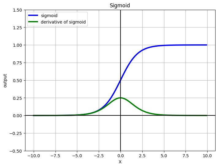

2. The Decision Boundary¶

The model predicts class 1 when $\sigma(z) \geq 0.5$ , which happens when $z \geq 0$ :

\boldsymbol{\theta}^\top \mathbf{x} + b \geq 0 \implies \hat{y} = 1

(2)

The decision boundary is the hyperplane $\boldsymbol{\theta}^\top \mathbf{x} + b = 0$ . In 2D this is a line; in $p$ dimensions it is a $(p-1)$ -dimensional hyperplane.

Non-linear boundaries are possible by adding polynomial or interaction features before fitting — logistic regression itself is always a linear classifier in the transformed feature space.

3. Binary Cross-Entropy Loss¶

Why not use MSE? MSE applied to a sigmoid output creates a non-convex loss surface — many local minima, poor gradients near 0 and 1.

Binary cross-entropy (BCE) is the correct loss for binary classification:

J(\boldsymbol{\theta}) = -\frac{1}{n} \sum_{i=1}^n \left[ y^{(i)} \log \hat{y}^{(i)} + (1 - y^{(i)}) \log(1 - \hat{y}^{(i)}) \right]

(3)

When $y = 1$ : loss $= -\log(\hat{y})$ — penalises low predicted probability
When $y = 0$ : loss $= -\log(1 - \hat{y})$ — penalises high predicted probability

The combined loss is convex when composed with the sigmoid, guaranteeing a unique global minimum.

Entropy and log-loss. Shannon entropy $H(p) = -p\log_2 p - (1-p)\log_2(1-p)$ measures uncertainty of a distribution. Log-loss measures how far our predicted distribution is from the true labels — it equals the cross-entropy between the empirical distribution (labels) and the model’s predicted distribution.

%matplotlib inline
import numpy as np
import matplotlib.pyplot as plt

def sigmoid(x):
    return 1 / (1 + np.exp(-x))

def entropy(p):
    p = np.clip(p, 1e-10, 1 - 1e-10)
    return -p * np.log2(p) - (1 - p) * np.log2(1 - p)

def log_loss(y_true, y_pred):
    y_pred = np.clip(y_pred, 1e-10, 1 - 1e-10)
    return - (y_true * np.log(y_pred) + (1 - y_true) * np.log(1 - y_pred))

fig, axes = plt.subplots(1, 3, figsize=(15, 4))

X = np.arange(-5, 5, 0.01)
axes[0].plot(sigmoid(X), -np.log(sigmoid(X)), c='blue', linewidth=3)
axes[0].set_xlabel('Sigmoid(X)')
axes[0].set_ylabel('-log(Sigmoid(X))')
axes[0].set_title('BCE loss when y = 1')
axes[0].grid(True)

X = np.arange(-10, 10, 0.01)
axes[1].plot(sigmoid(X), -np.log(1 - sigmoid(X)), c='red', linewidth=3)
axes[1].set_xlabel('Sigmoid(X)')
axes[1].set_ylabel('-log(1 - Sigmoid(X))')
axes[1].set_title('BCE loss when y = 0')
axes[1].grid(True)

p_vals = np.linspace(0.001, 0.999, 100)
axes[2].plot(p_vals, entropy(p_vals), c='purple', linewidth=3)
axes[2].set_xlabel('Probability (p)')
axes[2].set_ylabel('Entropy (bits)')
axes[2].set_title('Entropy of a binary distribution')
axes[2].grid(True)

plt.tight_layout()
plt.show()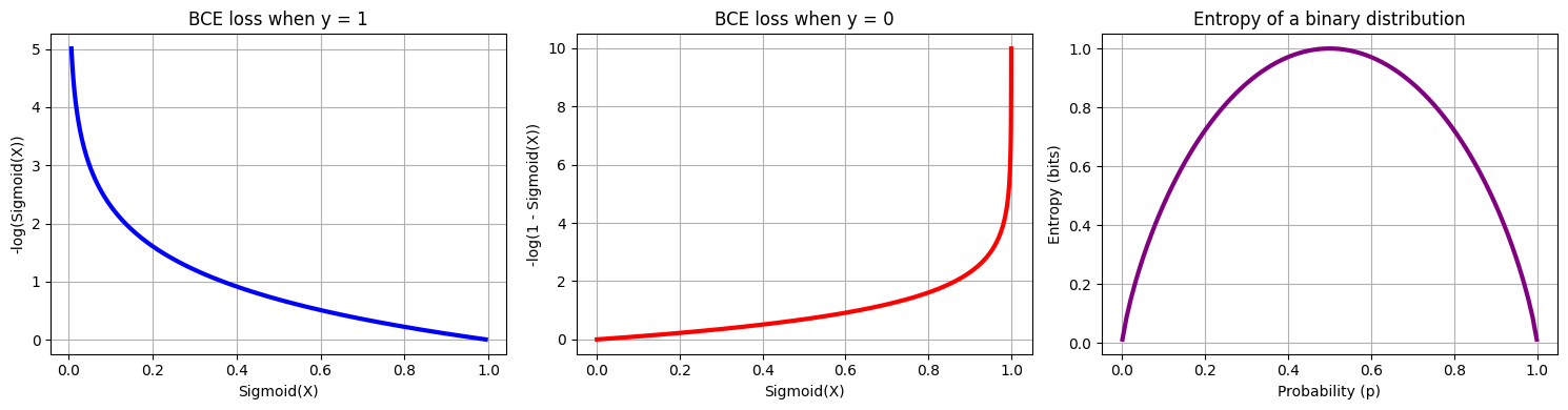

4. Gradient of the BCE Loss¶

With $\hat{y} = \sigma(\boldsymbol{\theta}^\top \mathbf{x} + b)$ , the gradient of BCE with respect to $\boldsymbol{\theta}$ is:

\frac{\partial J}{\partial \boldsymbol{\theta}} = \frac{1}{n} \mathbf{X}^\top (\hat{\mathbf{y}} - \mathbf{y})

(4)

\frac{\partial J}{\partial b} = \frac{1}{n} \sum_{i=1}^n (\hat{y}^{(i)} - y^{(i)})

(5)

This has the same form as the linear regression gradient — the model error $(\hat{y} - y)$ is back-propagated through the features. The sigmoid derivative cancels cleanly with the BCE terms.

Gradient update rule (same as previous notebooks):

\boldsymbol{\theta} \leftarrow \boldsymbol{\theta} - \alpha \cdot \frac{1}{n} \mathbf{X}^\top(\hat{\mathbf{y}} - \mathbf{y})

(6)

5. MLE vs MAP — From Probability to Regularisation¶

Maximum Likelihood Estimation (MLE) finds $\boldsymbol{\theta}$ that maximises the probability of observing the training labels:

\hat{\boldsymbol{\theta}}^{\text{MLE}} = \arg\max_\theta \prod_{i=1}^n P(y^{(i)} | \mathbf{x}^{(i)}, \boldsymbol{\theta})

(7)

Taking the negative log gives exactly the BCE loss — MLE = unregularised BCE minimisation.

Maximum A Posteriori (MAP) adds a prior over $\boldsymbol{\theta}$ . With a Gaussian prior $\boldsymbol{\theta} \sim \mathcal{N}(0, 1/\lambda)$ :

J_{\text{MAP}} = \underbrace{-\frac{1}{n}\sum_i [y^{(i)}\log\hat{y}^{(i)} + (1-y^{(i)})\log(1-\hat{y}^{(i)})]}_\text{BCE} + \underbrace{\frac{\lambda}{2n}\|\boldsymbol{\theta}\|^2}_\text{L2 penalty}

(8)

MAP + Gaussian prior = L2-regularised BCE.

Method	Objective	sklearn `C`	Behaviour
MLE	Pure BCE	$C \to \infty$	Unregularised, can overfit
MAP (Gaussian prior)	BCE + L2	$C = 1/\lambda$	Shrinks weights, reduces variance
MAP (Laplace prior)	BCE + L1	—	Sparse weights, feature selection

%matplotlib inline
import numpy as np
import matplotlib.pyplot as plt

# Coin flip MLE: dataset {H, H, T, H, T} — theta = P(H)
coin_likelihood = lambda theta: theta*theta*(1-theta)*theta*(1-theta)

theta_vals = np.linspace(0, 1, 200)
plt.figure(figsize=(7, 4))
plt.plot(theta_vals, coin_likelihood(theta_vals), linewidth=3, c='steelblue')
plt.scatter([0.6], [coin_likelihood(0.6)], color='red', s=100, zorder=5,
            label='MLE: theta=0.6 (3 heads / 5 flips)')
plt.xlabel('Parameter theta = P(Heads)')
plt.ylabel('Likelihood of the data')
plt.title('Coin Flip MLE — Data: {H, H, T, H, T}')
plt.legend()
plt.grid(True)
plt.show()

print('MLE estimate: theta = 3/5 =', 3/5, '(number of heads / total flips)')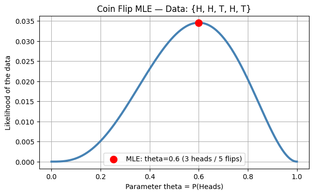

MLE estimate: theta = 3/5 = 0.6 (number of heads / total flips)

6. Weight Interpretation — Log-Odds and Odds Ratios¶

The log-odds (logit) of the model’s prediction is:

\log\frac{P(y=1|\mathbf{x})}{P(y=0|\mathbf{x})} = \boldsymbol{\theta}^\top \mathbf{x} + b = \theta_0 + \theta_1 x_1 + \theta_2 x_2 + \ldots

(9)

This is linear in the features. Each coefficient $\theta_j$ is the change in log-odds per unit increase in $x_j$ (all else held constant).

Odds ratio interpretation:

e^{\theta_j} = \text{odds ratio for } x_j

(10)

$e^{\theta_j} = 2$ : one unit increase in $x_j$ doubles the odds of class 1.
$e^{\theta_j} = 0.5$ : one unit increase halves the odds.
$e^{\theta_j} = 1$ : $x_j$ has no effect.

Important: always standardise features before interpreting magnitudes (coefficients only compare across features when features are on the same scale).

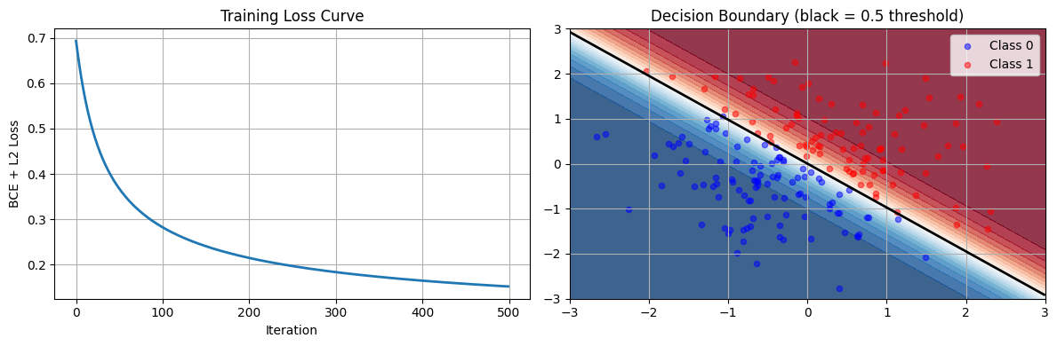
7. Logistic Regression from Scratch¶

The implementation below follows the GD loop from Chapter 6 — only the loss function and gradient change from linear regression.

%matplotlib inline
import numpy as np
import matplotlib.pyplot as plt

class LogisticRegression:
    def __init__(self, learning_rate=0.01, n_iterations=1000, lambda_reg=0.01):
        self.learning_rate = learning_rate
        self.n_iterations = n_iterations
        self.lambda_reg = lambda_reg
        self.weights = None
        self.bias = None
        self.losses = []

    def sigmoid(self, z):
        return 1 / (1 + np.exp(-z))

    def compute_loss(self, X, y, y_pred):
        N = len(y)
        cross_entropy = -np.mean(y * np.log(y_pred + 1e-15) + (1 - y) * np.log(1 - y_pred + 1e-15))
        l2_penalty = (self.lambda_reg / (2 * N)) * np.sum(self.weights ** 2)
        return cross_entropy + l2_penalty

    def fit(self, X, y):
        n_samples, n_features = X.shape
        self.weights = np.zeros(n_features)
        self.bias = 0

        for _ in range(self.n_iterations):
            linear_model = np.dot(X, self.weights) + self.bias
            y_pred = self.sigmoid(linear_model)

            loss = self.compute_loss(X, y, y_pred)
            self.losses.append(loss)

            dw = (1 / n_samples) * np.dot(X.T, (y_pred - y)) + (self.lambda_reg / n_samples) * self.weights
            db = (1 / n_samples) * np.sum(y_pred - y)

            self.weights -= self.learning_rate * dw
            self.bias -= self.learning_rate * db

    def predict_proba(self, X):
        linear_model = np.dot(X, self.weights) + self.bias
        return self.sigmoid(linear_model)

    def predict(self, X, threshold=0.5):
        return (self.predict_proba(X) >= threshold).astype(int)


np.random.seed(0)
X = np.random.randn(200, 2)
y = (X[:, 0] + X[:, 1] > 0).astype(int)

model = LogisticRegression(learning_rate=0.1, n_iterations=500, lambda_reg=0.1)
model.fit(X, y)

y_pred = model.predict(X)
accuracy = np.mean(y_pred == y)
print(f'Training accuracy: {accuracy:.4f}')
print(f'Final loss: {model.losses[-1]:.4f}')

fig, axes = plt.subplots(1, 2, figsize=(12, 4))

axes[0].plot(model.losses, linewidth=2)
axes[0].set_xlabel('Iteration')
axes[0].set_ylabel('BCE + L2 Loss')
axes[0].set_title('Training Loss Curve')
axes[0].grid(True)

xx, yy = np.meshgrid(np.linspace(-3, 3, 200), np.linspace(-3, 3, 200))
Z = model.predict_proba(np.c_[xx.ravel(), yy.ravel()]).reshape(xx.shape)
axes[1].contourf(xx, yy, Z, levels=20, cmap='RdBu_r', alpha=0.8)
axes[1].scatter(X[y==0, 0], X[y==0, 1], c='blue', alpha=0.5, label='Class 0', s=20)
axes[1].scatter(X[y==1, 0], X[y==1, 1], c='red', alpha=0.5, label='Class 1', s=20)
axes[1].contour(xx, yy, Z, levels=[0.5], colors='black', linewidths=2)
axes[1].set_title('Decision Boundary (black = 0.5 threshold)')
axes[1].legend()
axes[1].grid(True)

plt.tight_layout()
plt.show()

Training accuracy: 0.9950
Final loss: 0.1523

8. Try It in the Browser¶

Adjust the learning rate and regularisation strength to observe how training converges.

import math
import random

random.seed(42)

def sigmoid(z):
    return 1.0 / (1.0 + math.exp(-max(-500, min(500, z))))

n = 60
X = [random.gauss(-1, 1) for _ in range(n//2)] + [random.gauss(1, 1) for _ in range(n//2)]
y = [0] * (n//2) + [1] * (n//2)

lr = 0.5
lam = 0.01
w, b = 0.0, 0.0

for epoch in range(300):
    grad_w, grad_b = 0.0, 0.0
    loss = 0.0
    for xi, yi in zip(X, y):
        z = w * xi + b
        yhat = sigmoid(z)
        err = yhat - yi
        grad_w += err * xi
        grad_b += err
        eps = 1e-15
        loss -= yi * math.log(yhat + eps) + (1 - yi) * math.log(1 - yhat + eps)
    w -= lr * (grad_w / n + lam * w / n)
    b -= lr * grad_b / n
    loss /= n

correct = sum(1 for xi, yi in zip(X, y) if (sigmoid(w*xi + b) >= 0.5) == bool(yi))
decision_boundary = -b / w if w != 0 else float('nan')
print(f'w = {w:.4f}, b = {b:.4f}')
print(f'Decision boundary: x = {decision_boundary:.4f}')
print(f'Training accuracy: {correct/n:.1%}')
print(f'Final loss: {loss:.4f}')

9. Logistic Regression with scikit-learn¶

In practice use sklearn.linear_model.LogisticRegression. Note that sklearn’s C = 1/lambda — larger C means less regularisation.

%matplotlib inline
import numpy as np
import matplotlib.pyplot as plt
from sklearn.datasets import make_classification
from sklearn.linear_model import LogisticRegression as SklearnLR
from sklearn.model_selection import train_test_split
from sklearn.preprocessing import StandardScaler
from sklearn.metrics import accuracy_score, classification_report

X, y = make_classification(
    n_samples=1000, n_features=5, n_informative=3,
    n_redundant=1, random_state=42, class_sep=0.8
)
feature_names = ['monthly_charges', 'tenure', 'data_usage', 'support_calls', 'contract_length']

X_train, X_test, y_train, y_test = train_test_split(X, y, test_size=0.2, random_state=42)

scaler = StandardScaler()
X_train_s = scaler.fit_transform(X_train)
X_test_s = scaler.transform(X_test)

model_sk = SklearnLR(C=1.0, max_iter=1000, random_state=42)
model_sk.fit(X_train_s, y_train)

y_pred_sk = model_sk.predict(X_test_s)
print('Test accuracy:', accuracy_score(y_test, y_pred_sk))
print()
print(classification_report(y_test, y_pred_sk, target_names=['Stay', 'Churn']))

coefs = model_sk.coef_[0]
plt.figure(figsize=(7, 4))
colors = ['red' if c > 0 else 'steelblue' for c in coefs]
plt.barh(feature_names, coefs, color=colors)
plt.axvline(0, color='black', linewidth=0.8)
plt.xlabel('Log-odds coefficient')
plt.title('Logistic Regression Coefficients (standardised features)')
plt.grid(True, axis='x')
plt.tight_layout()
plt.show()

odds_ratios = np.exp(coefs)
print('\nOdds ratios:')
for name, OR in zip(feature_names, odds_ratios):
    print(f'  {name}: {OR:.3f}')

Test accuracy: 0.875

              precision    recall  f1-score   support

        Stay       0.80      0.95      0.87        87
       Churn       0.96      0.81      0.88       113

    accuracy                           0.88       200
   macro avg       0.88      0.88      0.87       200
weighted avg       0.89      0.88      0.88       200

/Volumes/MacSSD/01_Projects/Chandravesh-ML-Research/projects/jupyter-books/.venv/lib/python3.10/site-packages/sklearn/linear_model/_linear_loss.py:200: RuntimeWarning: divide by zero encountered in matmul
  raw_prediction = X @ weights + intercept
/Volumes/MacSSD/01_Projects/Chandravesh-ML-Research/projects/jupyter-books/.venv/lib/python3.10/site-packages/sklearn/linear_model/_linear_loss.py:200: RuntimeWarning: overflow encountered in matmul
  raw_prediction = X @ weights + intercept
/Volumes/MacSSD/01_Projects/Chandravesh-ML-Research/projects/jupyter-books/.venv/lib/python3.10/site-packages/sklearn/linear_model/_linear_loss.py:200: RuntimeWarning: invalid value encountered in matmul
  raw_prediction = X @ weights + intercept


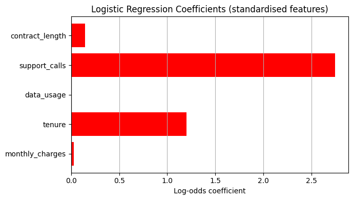
Odds ratios:
  monthly_charges: 1.030
  tenure: 3.318
  data_usage: 1.006
  support_calls: 15.614
  contract_length: 1.153

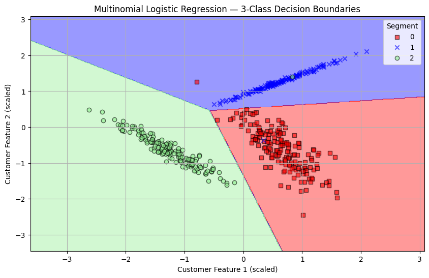
10. Softmax Regression — Generalising to K Classes¶

For $K > 2$ classes, the sigmoid is replaced by the softmax function:

P(y = k \mid \mathbf{x}) = \frac{e^{\boldsymbol{\theta}_k^\top \mathbf{x}}}{\sum_{l=1}^K e^{\boldsymbol{\theta}_l^\top \mathbf{x}}}

(11)

The loss becomes categorical cross-entropy:

J = -\frac{1}{n} \sum_{i=1}^n \sum_{k=1}^K y_k^{(i)} \log P(y=k \mid \mathbf{x}^{(i)})

(12)

where $y_k^{(i)}$ is the one-hot indicator for class $k$ .

Connection to logistic regression: with $K = 2$ , softmax reduces exactly to the sigmoid:

\frac{e^{\theta_1^\top \mathbf{x}}}{e^{\theta_1^\top \mathbf{x}} + e^{\theta_2^\top \mathbf{x}}} = \frac{1}{1 + e^{-(\theta_1 - \theta_2)^\top \mathbf{x}}} = \sigma((\boldsymbol{\theta}_1 - \boldsymbol{\theta}_2)^\top \mathbf{x})

(13)

The gradient is also clean: $\nabla_{\boldsymbol{\theta}_k} J = \frac{1}{n} \mathbf{X}^\top (\hat{\mathbf{P}}_k - \mathbf{y}_k)$ — same error-times-feature structure.

%matplotlib inline
import numpy as np
from scipy.special import softmax
from sklearn.preprocessing import LabelBinarizer
from sklearn.datasets import load_iris
from sklearn.model_selection import train_test_split
from sklearn.preprocessing import StandardScaler
from sklearn.metrics import accuracy_score

class SoftmaxRegression:
    def __init__(self, learning_rate=0.01, max_iter=1000, tol=1e-4, random_state=None):
        self.learning_rate = learning_rate
        self.max_iter = max_iter
        self.tol = tol
        self.random_state = random_state
        self.weights = None
        self.classes_ = None
        self.bias = None

    def _initialize_weights(self, n_features, n_classes):
        if self.random_state is not None:
            np.random.seed(self.random_state)
        self.weights = np.random.randn(n_features, n_classes) * 0.01
        self.bias = np.zeros(n_classes)

    def _one_hot_encode(self, y):
        self.label_binarizer = LabelBinarizer()
        return self.label_binarizer.fit_transform(y)

    def _gradient(self, X, y_true, y_pred):
        error = y_pred - y_true
        grad_weights = X.T @ error / X.shape[0]
        grad_bias = np.mean(error, axis=0)
        return grad_weights, grad_bias

    def fit(self, X, y):
        y_one_hot = self._one_hot_encode(y)
        self.classes_ = self.label_binarizer.classes_
        n_samples, n_features = X.shape
        n_classes = y_one_hot.shape[1]
        self._initialize_weights(n_features, n_classes)
        prev_loss = float('inf')

        for i in range(self.max_iter):
            logits = X @ self.weights + self.bias
            y_pred = softmax(logits, axis=1)
            loss = -np.mean(np.sum(y_one_hot * np.log(y_pred + 1e-15), axis=1))
            if np.abs(prev_loss - loss) < self.tol:
                print(f'Converged at iteration {i}')
                break
            prev_loss = loss
            grad_weights, grad_bias = self._gradient(X, y_one_hot, y_pred)
            self.weights -= self.learning_rate * grad_weights
            self.bias -= self.learning_rate * grad_bias

    def predict_proba(self, X):
        logits = X @ self.weights + self.bias
        return softmax(logits, axis=1)

    def predict(self, X):
        return self.classes_[np.argmax(self.predict_proba(X), axis=1)]


iris = load_iris()
X_iris, y_iris = iris.data, iris.target
X_train_i, X_test_i, y_train_i, y_test_i = train_test_split(X_iris, y_iris, test_size=0.2, random_state=42)

scaler_i = StandardScaler()
X_train_i = scaler_i.fit_transform(X_train_i)
X_test_i = scaler_i.transform(X_test_i)

softmax_model = SoftmaxRegression(learning_rate=0.1, max_iter=2000, tol=1e-5, random_state=42)
softmax_model.fit(X_train_i, y_train_i)

y_pred_soft = softmax_model.predict(X_test_i)
print(f'Iris test accuracy: {accuracy_score(y_test_i, y_pred_soft):.4f}')

Iris test accuracy: 1.0000

%matplotlib inline
import numpy as np
import matplotlib.pyplot as plt
from matplotlib.colors import ListedColormap
from sklearn.datasets import make_classification
from sklearn.linear_model import LogisticRegression
from sklearn.preprocessing import StandardScaler

def plot_decision_regions(X, y, model, resolution=0.02):
    markers = ('s', 'x', 'o', '^', 'v')
    colors = ('red', 'blue', 'lightgreen', 'gray', 'cyan')
    cmap = ListedColormap(colors[:len(np.unique(y))])
    x1_min, x1_max = X[:, 0].min() - 1, X[:, 0].max() + 1
    x2_min, x2_max = X[:, 1].min() - 1, X[:, 1].max() + 1
    xx1, xx2 = np.meshgrid(np.arange(x1_min, x1_max, resolution),
                           np.arange(x2_min, x2_max, resolution))
    Z = model.predict(np.array([xx1.ravel(), xx2.ravel()]).T)
    Z = Z.reshape(xx1.shape)
    plt.contourf(xx1, xx2, Z, alpha=0.4, cmap=cmap)
    plt.xlim(xx1.min(), xx1.max())
    plt.ylim(xx2.min(), xx2.max())
    for idx, cl in enumerate(np.unique(y)):
        plt.scatter(x=X[y == cl, 0], y=X[y == cl, 1],
                    alpha=0.6, c=cmap(idx), edgecolor='black',
                    marker=markers[idx], label=cl)

X_3, Y_3 = make_classification(
    n_samples=500, n_features=2, n_redundant=0,
    n_clusters_per_class=1, n_classes=3, class_sep=2.0, random_state=42
)
scaler_3 = StandardScaler()
X_3 = scaler_3.fit_transform(X_3)

logreg = LogisticRegression(C=1e5, multi_class='multinomial', solver='lbfgs')
logreg.fit(X_3, Y_3)

plt.figure(figsize=(10, 6))
plot_decision_regions(X_3, Y_3, logreg)
plt.xlabel('Customer Feature 1 (scaled)')
plt.ylabel('Customer Feature 2 (scaled)')
plt.title('Multinomial Logistic Regression — 3-Class Decision Boundaries')
plt.legend(title='Segment')
plt.grid(True)
plt.show()

/Volumes/MacSSD/01_Projects/Chandravesh-ML-Research/projects/jupyter-books/.venv/lib/python3.10/site-packages/sklearn/linear_model/_logistic.py:1272: FutureWarning: 'multi_class' was deprecated in version 1.5 and will be removed in 1.8. From then on, it will always use 'multinomial'. Leave it to its default value to avoid this warning.
  warnings.warn(
/Volumes/MacSSD/01_Projects/Chandravesh-ML-Research/projects/jupyter-books/.venv/lib/python3.10/site-packages/sklearn/utils/extmath.py:203: RuntimeWarning: divide by zero encountered in matmul
  ret = a @ b
/Volumes/MacSSD/01_Projects/Chandravesh-ML-Research/projects/jupyter-books/.venv/lib/python3.10/site-packages/sklearn/utils/extmath.py:203: RuntimeWarning: overflow encountered in matmul
  ret = a @ b
/Volumes/MacSSD/01_Projects/Chandravesh-ML-Research/projects/jupyter-books/.venv/lib/python3.10/site-packages/sklearn/utils/extmath.py:203: RuntimeWarning: invalid value encountered in matmul
  ret = a @ b
/var/folders/93/7lt42x5j7m39kz7wxbcghvrm0000gn/T/ipykernel_68071/274246045.py:23: UserWarning: *c* argument looks like a single numeric RGB or RGBA sequence, which should be avoided as value-mapping will have precedence in case its length matches with *x* & *y*.  Please use the *color* keyword-argument or provide a 2D array with a single row if you intend to specify the same RGB or RGBA value for all points.
  plt.scatter(x=X[y == cl, 0], y=X[y == cl, 1],
/var/folders/93/7lt42x5j7m39kz7wxbcghvrm0000gn/T/ipykernel_68071/274246045.py:23: UserWarning: You passed a edgecolor/edgecolors ('black') for an unfilled marker ('x').  Matplotlib is ignoring the edgecolor in favor of the facecolor.  This behavior may change in the future.
  plt.scatter(x=X[y == cl, 0], y=X[y == cl, 1],

Knowledge Check¶

Why is logistic regression used for binary classification instead of plain linear regression?¶

Because binary classification has no featuresBinary tasks still use features as inputs.

Because logistic regression maps the linear score into a probability between 0 and 1Correct. The sigmoid link makes the output suitable for binary probability interpretation.

Because linear regression cannot use coefficientsLinear regression also uses coefficients.

Because logistic regression never needs data preprocessingPreprocessing can still matter.

What does the decision threshold do in logistic regression?¶

It converts predicted probabilities into class labelsCorrect. The threshold determines when the model predicts the positive class.

It removes the sigmoid functionThe threshold is applied after the probability is produced.

It estimates the regression interceptThe intercept is learned during model fitting.

It sets the number of input featuresFeature count comes from the dataset design.

Minimising binary cross-entropy is equivalent to which statistical estimation principle?¶

Minimising mean squared errorMSE is the objective for linear regression, not logistic.

Maximum Likelihood Estimation (MLE)Correct. Negative log-likelihood equals BCE for Bernoulli-distributed labels.

Minimising entropy of the predictionEntropy of predictions is not the training objective here.

Maximising model complexityThe objective is data fit, not complexity.

If a logistic regression weight for feature x is theta = 0.693, the exponentiated odds ratio exp(theta) ≈ 2. What does this mean?¶

The probability of class 1 doubles for each unit increase in xThe probability change depends on the base rate — only the odds double.

The odds of class 1 double for each unit increase in xCorrect. exp(theta) is the multiplicative change in odds, not probability.

The feature x is twice as important as any other featureImportance also depends on feature scale and other weights.

The model accuracy doublesOdds ratio is about prediction, not global accuracy.

Exercises¶

Exercise 1 — Threshold Tuning¶

Using the LogisticRegression model trained on the churn dataset above, plot precision, recall, and F1 score as a function of threshold (sweep from 0.1 to 0.9 in steps of 0.05). Identify the threshold that maximises F1.

%matplotlib inline
# Exercise 1: threshold tuning
# Your code here

Exercise 2 — Regularisation Strength¶

Sweep lambda_reg over [0.001, 0.01, 0.1, 1.0, 10.0] in your scratch LogisticRegression. For each value, fit on 80 % of the synthetic dataset and compute test accuracy. Plot accuracy vs log(lambda). At what lambda does the model start to underfit?

%matplotlib inline
# Exercise 2: regularisation sweep
# Your code here

Common Pitfalls¶

What’s Next?¶

Logistic regression assumes features are roughly independent — it builds a single linear boundary. In Naive Bayes (naive_bayes.ipynb) we approach classification from a probabilistic generative model angle, explicitly modelling the class-conditional feature distributions and using Bayes’ theorem to derive the posterior.

Coming up in Chapter 7:

Naive Bayes — Bayes’ theorem, class-conditional independence, Gaussian vs Multinomial NB
Calibration & Class Imbalance — reliability diagrams, SMOTE, cost-sensitive learning
Classification Metrics — precision, recall, F1, AUC-ROC, AUC-PR
Lab — Churn Prediction end-to-end pipeline