
Lab - Fraud Detection with Tree Ensembles
Lab goal: build an end-to-end fraud classifier using Decision Tree, Random Forest, and Gradient Boosting; evaluate with imbalanced-data metrics; and interpret business decisions with feature importance.
Business Brief
A payments team wants to reduce fraudulent transactions without blocking too many legitimate customers. False negatives are expensive (missed fraud), but false positives also hurt user experience.
Continuity from feature_importance.ipynb
In the previous notebook, you learned how to interpret feature importance. This lab asks you to apply those ideas on a full training-and-evaluation workflow.
1. Workflow Overview
2. Why This Lab Uses a Synthetic Dataset
To keep this notebook reproducible in any environment, we generate a realistic synthetic fraud dataset with:
severe class imbalance
behavioral features (
amount,hour,velocity_1h,country_risk, etc.)latent fraud patterns plus noise
This allows you to run the full lab without dependency on external file availability.
3. Build Dataset + Train Baseline Models
%matplotlib inline
import numpy as np
import pandas as pd
import matplotlib.pyplot as plt

from sklearn.model_selection import train_test_split
from sklearn.tree import DecisionTreeClassifier
from sklearn.ensemble import RandomForestClassifier, GradientBoostingClassifier
from sklearn.metrics import (
    classification_report,
    roc_auc_score,
    average_precision_score,
    precision_recall_curve,
)

rng = np.random.default_rng(42)
n = 12000

# Synthetic transaction features
amount = rng.lognormal(mean=3.1, sigma=0.9, size=n)
hour = rng.integers(0, 24, size=n)
country_risk = rng.beta(2.0, 5.0, size=n)
velocity_1h = rng.poisson(1.3, size=n)
merchant_risk = rng.beta(2.5, 3.5, size=n)
account_age_days = rng.integers(1, 2500, size=n)
device_trust = rng.beta(3.0, 2.5, size=n)

# Fraud propensity: nonlinear + interaction effects
score = (
    0.0028 * amount
    + 0.9 * country_risk
    + 0.45 * merchant_risk
    + 0.34 * velocity_1h
    - 0.00045 * account_age_days
    - 0.8 * device_trust
    + 0.22 * ((hour <= 5) | (hour >= 23)).astype(float)
)

prob = 1 / (1 + np.exp(-(score - 3.8)))
y = rng.binomial(1, np.clip(prob, 0, 1))

# Force stronger imbalance close to real fraud settings
mask_keep = (y == 0) | (rng.random(n) < 0.32)

X = pd.DataFrame(
    {
        "amount": amount,
        "hour": hour,
        "country_risk": country_risk,
        "velocity_1h": velocity_1h,
        "merchant_risk": merchant_risk,
        "account_age_days": account_age_days,
        "device_trust": device_trust,
    }
).loc[mask_keep].reset_index(drop=True)
y = y[mask_keep]

print(f"Samples: {len(X):,}")
print(f"Fraud rate: {y.mean()*100:.2f}%")

X_train, X_test, y_train, y_test = train_test_split(
    X, y, test_size=0.3, random_state=42, stratify=y
)

models = {
    "Decision Tree": DecisionTreeClassifier(max_depth=6, min_samples_leaf=20, random_state=42),
    "Random Forest": RandomForestClassifier(
        n_estimators=320,
        max_depth=8,
        min_samples_leaf=8,
        random_state=42,
        n_jobs=-1,
    ),
    "Gradient Boosting": GradientBoostingClassifier(
        n_estimators=260,
        learning_rate=0.05,
        max_depth=3,
        random_state=42,
    ),
}

rows = []
probas = {}
for name, model in models.items():
    model.fit(X_train, y_train)
    p = model.predict_proba(X_test)[:, 1]
    y_hat = (p >= 0.5).astype(int)
    probas[name] = p
    rows.append(
        {
            "model": name,
            "roc_auc": roc_auc_score(y_test, p),
            "pr_auc": average_precision_score(y_test, p),
            "f1_at_0.5": classification_report(y_test, y_hat, output_dict=True)["1"]["f1-score"],
        }
    )

results = pd.DataFrame(rows).sort_values("pr_auc", ascending=False)
print("\nModel comparison:")
print(results.round(4).to_string(index=False))
Samples: 11,774
Fraud rate: 0.92%
/Volumes/MacSSD/01_Projects/Chandravesh-ML-Research/projects/jupyter-books/.venv/lib/python3.10/site-packages/sklearn/metrics/_classification.py:1731: UndefinedMetricWarning: Precision is ill-defined and being set to 0.0 in labels with no predicted samples. Use `zero_division` parameter to control this behavior.
  _warn_prf(average, modifier, f"{metric.capitalize()} is", result.shape[0])
Model comparison:
            model  roc_auc  pr_auc  f1_at_0.5
Gradient Boosting   0.5418  0.0134        0.0
    Random Forest   0.5579  0.0120        0.0
    Decision Tree   0.5401  0.0109        0.0
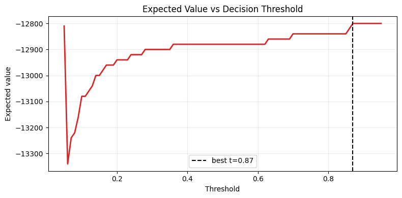
4. Threshold Tuning by Business Value
Fraud models should not always use a fixed 0.50 threshold. We optimize for expected value:
Use this section to find the threshold that maximizes business benefit on validation/test data.
%matplotlib inline
import numpy as np
import matplotlib.pyplot as plt
from sklearn.metrics import confusion_matrix

best_model_name = results.iloc[0]["model"]
p_best = probas[best_model_name]

thresholds = np.linspace(0.05, 0.95, 91)
value_tp, cost_fp, cost_fn = 250.0, 20.0, 400.0

evs = []
for t in thresholds:
    y_hat = (p_best >= t).astype(int)
    tn, fp, fn, tp = confusion_matrix(y_test, y_hat).ravel()
    ev = tp * value_tp - fp * cost_fp - fn * cost_fn
    evs.append(ev)

best_idx = int(np.argmax(evs))
best_t = thresholds[best_idx]
print(f"Best model by PR-AUC: {best_model_name}")
print(f"Best threshold by EV: {best_t:.2f}")
print(f"Max expected value: {evs[best_idx]:,.0f}")

plt.figure(figsize=(8, 4))
plt.plot(thresholds, evs, color="#d62828", lw=2)
plt.axvline(best_t, linestyle="--", color="black", label=f"best t={best_t:.2f}")
plt.title("Expected Value vs Decision Threshold")
plt.xlabel("Threshold")
plt.ylabel("Expected value")
plt.grid(alpha=0.25)
plt.legend()
plt.tight_layout()
plt.show()
Best model by PR-AUC: Gradient Boosting
Best threshold by EV: 0.87
Max expected value: -12,800
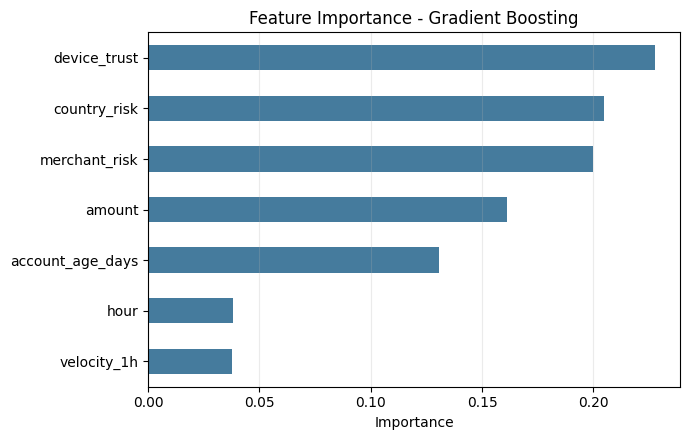
5. Feature Importance (Lab Interpretation)
We inspect top features from the best-performing model and convert them into action points for risk operations.
%matplotlib inline
import pandas as pd
import matplotlib.pyplot as plt

best_model = models[best_model_name]
imp = pd.Series(best_model.feature_importances_, index=X.columns).sort_values(ascending=False)
print("Top feature importances:")
print(imp.head(7).round(4).to_string())

plt.figure(figsize=(7, 4.5))
imp.sort_values().plot.barh(color="#457b9d")
plt.title(f"Feature Importance - {best_model_name}")
plt.xlabel("Importance")
plt.grid(axis="x", alpha=0.25)
plt.tight_layout()
plt.show()
Top feature importances:
device_trust 0.2275
country_risk 0.2049
merchant_risk 0.1999
amount 0.1612
account_age_days 0.1306
hour 0.0382
velocity_1h 0.0376
6. Try It in the Browser
A tiny EV calculator for threshold decisions.
def expected_value(tp, fp, fn, value_tp=250, cost_fp=20, cost_fn=400):
    return tp * value_tp - fp * cost_fp - fn * cost_fn

scenario_A = {"tp": 42, "fp": 120, "fn": 18}
scenario_B = {"tp": 35, "fp": 60, "fn": 25}

print("Scenario A EV:", expected_value(**scenario_A))
print("Scenario B EV:", expected_value(**scenario_B))
print("Choose the scenario with higher EV, not necessarily higher precision alone.")
Knowledge Check
Why is PR-AUC often preferred over accuracy in fraud detection?
CheckA threshold that maximizes expected value should be selected using:
CheckExercises
Exercise 1 - Model extension
Add class_weight='balanced' to the Decision Tree and Random Forest models. Compare PR-AUC and EV.
Exercise 2 - Calibration test
Calibrate the best model (CalibratedClassifierCV) and re-run threshold optimization.
Exercise 3 - Operations memo
Write a one-page recommendation: selected model, selected threshold, projected EV impact, and top-3 risk drivers.
Summary
Tree ensembles improve fraud detection over single trees.
In imbalanced data, PR-AUC and business EV are stronger decision metrics than accuracy.
Threshold tuning can materially change business outcomes.
Feature importance translates model behavior into actionable risk controls.

What’s Next - Unsupervised Learning
Next, move to unsupervised.ipynb, where you will analyze structure without labels (PCA, clustering, and dimensionality reduction).