Decision Trees — Splits, Impurity, and Interpretable Models¶

What you will learn: how decision trees split data to minimise impurity (entropy/Gini for classification, variance for regression), the ID3/CART algorithm, information gain, how depth controls bias-variance, pruning strategies, and how to implement a decision tree from scratch.

Why Decision Trees Matter for Business¶

A bank’s credit risk model must be explainable to regulators: “Customer rejected because: income < £25k AND credit history < 3 years.” Decision trees produce rules that compliance officers can read directly. No other ML model achieves this combination of predictive power and transparency.

A Decision Tree builds exactly this rule structure automatically from labelled training data.

Continuity from KNN¶

In knn_lab.ipynb, predictions came from distance to neighbours and required feature scaling. Trees switch to axis-aligned threshold rules (for example, income <= 30000), so they are naturally scale-invariant and easier to explain to non-technical stakeholders.

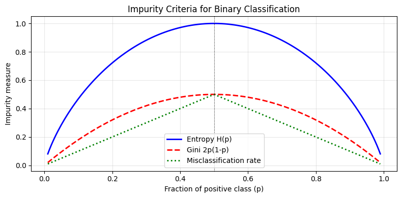
1. Splitting Criteria — Measuring Impurity¶

The tree chooses splits that maximally reduce impurity in the child nodes.

Entropy (ID3)¶

H(S) = -\sum_{k=1}^{K} p_k \log_2 p_k

(1)

Information Gain:

IG(S, f, t) = H(S) - \frac{|S_L|}{|S|} H(S_L) - \frac{|S_R|}{|S|} H(S_R)

(2)

Gini Impurity (CART)¶

G(S) = 1 - \sum_{k=1}^{K} p_k^2

(3)

Gini is faster to compute (no log) and gives similar results to entropy. sklearn uses Gini by default.

Variance Reduction (Regression CART)¶

\text{Gain} = \text{Var}(S) - \frac{|S_L|}{|S|} \text{Var}(S_L) - \frac{|S_R|}{|S|} \text{Var}(S_R)

(4)

Criterion	Task	Range	Notes
Entropy	Classification	[0, log₂K]	Slightly higher complexity, similar performance
Gini	Classification	[0, 1)	Faster, sklearn default
Variance	Regression	[0, ∞)	Equivalent to MSE reduction

%matplotlib inline
import numpy as np
import matplotlib.pyplot as plt

p = np.linspace(0.01, 0.99, 200)

entropy_val = -p * np.log2(p) - (1 - p) * np.log2(1 - p)
gini_val = 2 * p * (1 - p)  # binary Gini = 1 - p² - (1-p)²
misclassif = 1 - np.maximum(p, 1 - p)

fig, ax = plt.subplots(figsize=(8, 4))
ax.plot(p, entropy_val, 'b-', lw=2, label='Entropy H(p)')
ax.plot(p, gini_val, 'r--', lw=2, label='Gini 2p(1-p)')
ax.plot(p, misclassif, 'g:', lw=2, label='Misclassification rate')
ax.axvline(0.5, color='k', lw=0.8, linestyle=':')
ax.set_xlabel('Fraction of positive class (p)')
ax.set_ylabel('Impurity measure')
ax.set_title('Impurity Criteria for Binary Classification')
ax.legend(); ax.grid(alpha=0.3)
plt.tight_layout()
plt.show()

# Numerical example
print("Example: node with 10 samples, 7 positives, 3 negatives")
p_val = 7/10
h = -(p_val * np.log2(p_val) + (1-p_val) * np.log2(1-p_val))
g = 1 - p_val**2 - (1-p_val)**2
print(f"  Entropy = {h:.4f}")
print(f"  Gini    = {g:.4f}")
print(f"  Misclassification = {1 - max(p_val, 1-p_val):.4f}")

Example: node with 10 samples, 7 positives, 3 negatives
  Entropy = 0.8813
  Gini    = 0.4200
  Misclassification = 0.3000

2. Decision Tree from Scratch¶

The implementation below supports both classification (entropy/information gain) and regression (variance reduction). It preserves all the original user-written code.

%matplotlib inline
import numpy as np
import matplotlib.pyplot as plt
from collections import Counter
from sklearn.datasets import make_regression, load_iris
from sklearn.model_selection import train_test_split
from sklearn.metrics import accuracy_score, mean_squared_error


def entropy(y):
    hist = np.bincount(y)
    ps = hist / len(y)
    return -np.sum([p * np.log2(p) for p in ps if p > 0])

def variance(y):
    return np.var(y) if len(y) > 0 else 0

def information_gain(X, y, feature_idx, threshold):
    parent_entropy = entropy(y)
    left_mask = X[:, feature_idx] <= threshold
    right_mask = ~left_mask
    if np.sum(left_mask) == 0 or np.sum(right_mask) == 0:
        return 0
    n = len(y)
    n_left, n_right = np.sum(left_mask), np.sum(right_mask)
    child_entropy = (n_left / n) * entropy(y[left_mask]) + (n_right / n) * entropy(y[right_mask])
    return parent_entropy - child_entropy

def variance_reduction(X, y, feature_idx, threshold):
    parent_var = variance(y)
    left_mask = X[:, feature_idx] <= threshold
    right_mask = ~left_mask
    if np.sum(left_mask) == 0 or np.sum(right_mask) == 0:
        return 0
    n = len(y)
    n_left, n_right = np.sum(left_mask), np.sum(right_mask)
    child_var = (n_left / n) * variance(y[left_mask]) + (n_right / n) * variance(y[right_mask])
    return parent_var - child_var


class Node:
    def __init__(self, feature_idx=None, threshold=None, left=None, right=None, value=None):
        self.feature_idx = feature_idx
        self.threshold = threshold
        self.left = left
        self.right = right
        self.value = value


class DecisionTree:
    def __init__(self, max_depth=3, min_samples_split=2, criterion='entropy'):
        self.max_depth = max_depth
        self.min_samples_split = min_samples_split
        self.criterion = criterion
        self.root = None
        self.boundaries = []

    def fit(self, X, y):
        self.root = self._grow_tree(X, y, depth=0)

    def _grow_tree(self, X, y, depth):
        n_samples, n_features = X.shape
        if depth >= self.max_depth or n_samples < self.min_samples_split:
            return Node(value=self._leaf_value(y))
        best_gain = -1
        best_idx, best_threshold = None, None
        for feature_idx in range(n_features):
            thresholds = np.unique(X[:, feature_idx])
            for threshold in thresholds:
                gain = (information_gain(X, y, feature_idx, threshold)
                        if self.criterion == 'entropy'
                        else variance_reduction(X, y, feature_idx, threshold))
                if gain > best_gain:
                    best_gain = gain
                    best_idx = feature_idx
                    best_threshold = threshold
        if best_gain <= 0:
            return Node(value=self._leaf_value(y))
        self.boundaries.append((best_idx, best_threshold, depth))
        left_mask = X[:, best_idx] <= best_threshold
        left = self._grow_tree(X[left_mask], y[left_mask], depth + 1)
        right = self._grow_tree(X[~left_mask], y[~left_mask], depth + 1)
        return Node(best_idx, best_threshold, left, right)

    def _leaf_value(self, y):
        return Counter(y).most_common(1)[0][0] if self.criterion == 'entropy' else np.mean(y)

    def predict(self, X):
        return np.array([self._predict(x, self.root) for x in X])

    def _predict(self, x, node):
        if node.value is not None:
            return node.value
        if x[node.feature_idx] <= node.threshold:
            return self._predict(x, node.left)
        return self._predict(x, node.right)

    def get_prediction_path(self, x):
        path = []
        node = self.root
        while node.value is None:
            path.append((node.feature_idx, node.threshold))
            node = node.left if x[node.feature_idx] <= node.threshold else node.right
        path.append(('leaf', node.value))
        return path


# --- Classification: Iris ---
from sklearn.datasets import load_iris
iris = load_iris()
X_tr, X_te, y_tr, y_te = train_test_split(iris.data, iris.target, test_size=0.2, random_state=42)
clf = DecisionTree(max_depth=3, criterion='entropy')
clf.fit(X_tr, y_tr)
y_pred = clf.predict(X_te)
print(f"Classification Accuracy (Iris, depth=3): {accuracy_score(y_te, y_pred):.4f}")

# Path explanation for first test point
path = clf.get_prediction_path(X_te[0])
print(f"\nPrediction path for X_te[0] = {X_te[0]}:")
for step in path[:-1]:
    print(f"  Feature[{step[0]}] ({iris.feature_names[step[0]]}) <= {step[1]:.3f}?")
print(f"  → Leaf: class = {iris.target_names[int(path[-1][1])]}")

# --- Regression ---
X_r, y_r = make_regression(n_samples=100, n_features=4, noise=0.1, random_state=42)
X_tr_r, X_te_r, y_tr_r, y_te_r = train_test_split(X_r, y_r, test_size=0.2, random_state=42)
reg = DecisionTree(max_depth=3, criterion='variance')
reg.fit(X_tr_r, y_tr_r)
y_pred_r = reg.predict(X_te_r)
print(f"\nRegression MSE (depth=3): {mean_squared_error(y_te_r, y_pred_r):.4f}")

Classification Accuracy (Iris, depth=3): 0.9667

Prediction path for X_te[0] = [6.1 2.8 4.7 1.2]:
  Feature[2] (petal length (cm)) <= 1.900?
  Feature[2] (petal length (cm)) <= 4.700?
  Feature[3] (petal width (cm)) <= 1.600?
  → Leaf: class = versicolor

Regression MSE (depth=3): 2358.0187

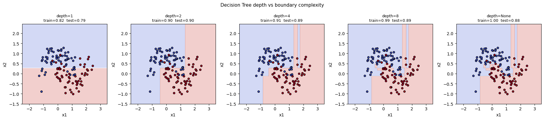
3. The Effect of max_depth on Bias-Variance¶

Deeper trees partition the space more finely. They reduce bias but increase variance — classic overfitting as depth → unlimited.

%matplotlib inline
import numpy as np
import matplotlib.pyplot as plt
from sklearn.tree import DecisionTreeClassifier
from sklearn.datasets import make_moons
from sklearn.model_selection import train_test_split
from sklearn.metrics import accuracy_score

np.random.seed(42)
X, y = make_moons(n_samples=400, noise=0.25, random_state=42)
X_tr, X_te, y_tr, y_te = train_test_split(X, y, test_size=0.3, random_state=42)

depths = [1, 2, 4, 8, None]
fig, axes = plt.subplots(1, len(depths), figsize=(18, 4))
h = 0.04
xx, yy = np.meshgrid(np.arange(-2.5, 3.5, h), np.arange(-1.5, 2.5, h))

for ax, d in zip(axes, depths):
    dt = DecisionTreeClassifier(max_depth=d, random_state=42)
    dt.fit(X_tr, y_tr)
    Z = dt.predict(np.c_[xx.ravel(), yy.ravel()]).reshape(xx.shape)
    ax.contourf(xx, yy, Z, cmap=plt.cm.coolwarm, alpha=0.25)
    ax.scatter(X_te[:,0], X_te[:,1], c=y_te, cmap=plt.cm.coolwarm, edgecolors='k', s=20)
    tr_acc = accuracy_score(y_tr, dt.predict(X_tr))
    te_acc = accuracy_score(y_te, dt.predict(X_te))
    label = f"depth={d}" if d else "depth=None"
    ax.set_title(f"{label}\ntrain={tr_acc:.2f}  test={te_acc:.2f}", fontsize=9)
    ax.set_xlabel('x1'); ax.set_ylabel('x2')

plt.suptitle('Decision Tree depth vs boundary complexity', fontsize=11)
plt.tight_layout()
plt.show()

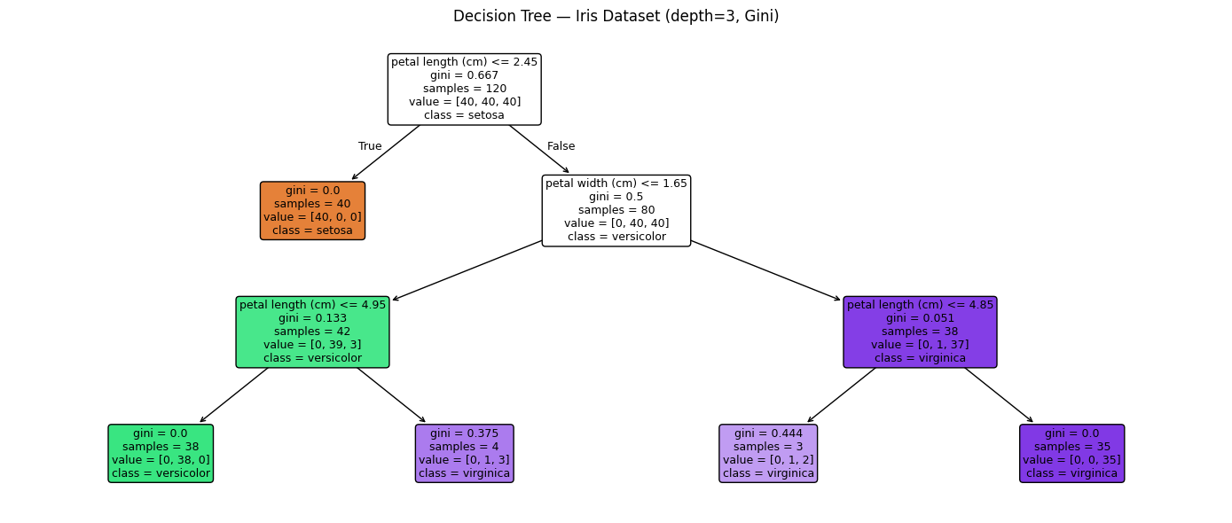
4. sklearn DecisionTree and Tree Visualisation¶

%matplotlib inline
import numpy as np
import matplotlib.pyplot as plt
from sklearn.tree import DecisionTreeClassifier, plot_tree, export_text
from sklearn.datasets import load_iris
from sklearn.model_selection import train_test_split
from sklearn.metrics import classification_report

iris = load_iris()
X_tr, X_te, y_tr, y_te = train_test_split(iris.data, iris.target,
                                            test_size=0.2, random_state=42, stratify=iris.target)

dt = DecisionTreeClassifier(max_depth=3, criterion='gini', random_state=42)
dt.fit(X_tr, y_tr)
y_pred = dt.predict(X_te)

print("=== sklearn Decision Tree (Iris, Gini, depth=3) ===")
print(classification_report(y_te, y_pred, target_names=iris.target_names))

# Text representation
print("\nTree rules:")
print(export_text(dt, feature_names=list(iris.feature_names)))

# Plot tree
fig, ax = plt.subplots(figsize=(14, 6))
plot_tree(dt, feature_names=iris.feature_names,
          class_names=iris.target_names,
          filled=True, rounded=True, ax=ax, fontsize=9)
ax.set_title('Decision Tree — Iris Dataset (depth=3, Gini)', fontsize=12)
plt.tight_layout()
plt.show()

=== sklearn Decision Tree (Iris, Gini, depth=3) ===
              precision    recall  f1-score   support

      setosa       1.00      1.00      1.00        10
  versicolor       1.00      0.90      0.95        10
   virginica       0.91      1.00      0.95        10

    accuracy                           0.97        30
   macro avg       0.97      0.97      0.97        30
weighted avg       0.97      0.97      0.97        30


Tree rules:
|--- petal length (cm) <= 2.45
|   |--- class: 0
|--- petal length (cm) >  2.45
|   |--- petal width (cm) <= 1.65
|   |   |--- petal length (cm) <= 4.95
|   |   |   |--- class: 1
|   |   |--- petal length (cm) >  4.95
|   |   |   |--- class: 2
|   |--- petal width (cm) >  1.65
|   |   |--- petal length (cm) <= 4.85
|   |   |   |--- class: 2
|   |   |--- petal length (cm) >  4.85
|   |   |   |--- class: 2

5. Pruning — Controlling Overfitting¶

Decision trees are prone to overfitting. Key hyperparameters for regularisation:

Parameter	Effect
`max_depth`	Hard stop on tree depth
`min_samples_split`	Minimum samples to consider a split
`min_samples_leaf`	Minimum samples per leaf node
`max_features`	Fraction of features to consider at each split
`ccp_alpha`	Cost-complexity pruning (higher = more pruning)

Cost-Complexity Pruning (CART): Minimise $R_\alpha(T) = R(T) + \alpha |T|$ where $R(T)$ is the tree’s training error and $|T|$ is the number of leaves. As $\alpha$ increases, smaller trees are preferred.

%matplotlib inline
import numpy as np
import matplotlib.pyplot as plt
from sklearn.tree import DecisionTreeClassifier
from sklearn.datasets import make_moons
from sklearn.model_selection import train_test_split, cross_val_score

np.random.seed(42)
X, y = make_moons(n_samples=500, noise=0.3, random_state=42)
X_tr, X_te, y_tr, y_te = train_test_split(X, y, test_size=0.3, random_state=42)

# CCP alpha path
path = DecisionTreeClassifier(random_state=42).cost_complexity_pruning_path(X_tr, y_tr)
alphas = path.ccp_alphas[:-1]  # last alpha gives a single-node tree

train_accs, test_accs = [], []
for alpha in alphas:
    dt = DecisionTreeClassifier(ccp_alpha=alpha, random_state=42)
    dt.fit(X_tr, y_tr)
    train_accs.append(dt.score(X_tr, y_tr))
    test_accs.append(dt.score(X_te, y_te))

best_alpha = alphas[np.argmax(test_accs)]
fig, ax = plt.subplots(figsize=(8, 4))
ax.semilogx(alphas, train_accs, 'b-o', markersize=3, label='Train accuracy')
ax.semilogx(alphas, test_accs, 'r-s', markersize=3, label='Test accuracy')
ax.axvline(best_alpha, color='k', linestyle='--', label=f'Best α={best_alpha:.5f}')
ax.set_xlabel('ccp_alpha (log scale)'); ax.set_ylabel('Accuracy')
ax.set_title('Cost-Complexity Pruning Path')
ax.legend(); ax.grid(alpha=0.3)
plt.tight_layout()
plt.show()
print(f"Best ccp_alpha = {best_alpha:.6f}  test accuracy = {max(test_accs):.4f}")

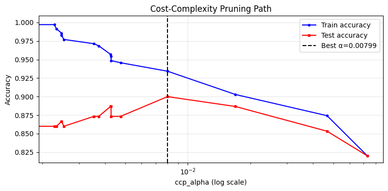
Best ccp_alpha = 0.007994  test accuracy = 0.9000

6. Try It in the Browser¶

Compute entropy and information gain for a simple binary split.

import math

def entropy(counts):
    total = sum(counts)
    if total == 0: return 0
    return -sum((c/total) * math.log2(c/total) for c in counts if c > 0)

def info_gain(parent, left, right):
    n = sum(parent)
    n_l, n_r = sum(left), sum(right)
    return entropy(parent) - (n_l/n)*entropy(left) - (n_r/n)*entropy(right)

# Parent node: 10 positives, 10 negatives
parent = [10, 10]
print(f"Parent entropy: {entropy(parent):.4f}  (max=1.0 for balanced)")

# Split A: left=[8pos,2neg], right=[2pos,8neg]
left_A, right_A = [8, 2], [2, 8]
print(f"\nSplit A: left={left_A}  right={right_A}")
print(f"  left entropy  = {entropy(left_A):.4f}")
print(f"  right entropy = {entropy(right_A):.4f}")
print(f"  IG = {info_gain(parent, left_A, right_A):.4f}")

# Split B: left=[10pos,5neg], right=[0pos,5neg]
left_B, right_B = [10, 5], [0, 5]
print(f"\nSplit B: left={left_B}  right={right_B}")
print(f"  left entropy  = {entropy(left_B):.4f}")
print(f"  right entropy = {entropy(right_B):.4f}")
print(f"  IG = {info_gain(parent, left_B, right_B):.4f}")
print("\nSplit B is better (purer right child)")

Knowledge Check¶

A leaf node with 15 positive and 15 negative samples has Gini impurity of:¶

[ ] A) 0.0 [ ] B) 0.5 — maximum Gini for a binary node [ ] C) 1.0 [ ] D) 0.25

Check

Decision trees are scale-invariant (no feature scaling needed) because:¶

[ ] A) They use cosine similarity instead of Euclidean distance [ ] B) Each split is a threshold comparison on a single feature — the decision depends only on the order of values, not their magnitudes [ ] C) They normalise features internally [ ] D) They use L1 regularisation which removes scale dependence

Check

Exercises¶

Exercise 1 — Hyperparameter Tuning¶

On make_moons(n_samples=600, noise=0.25), use GridSearchCV over max_depth ∈ [1,2,3,4,5,6,None] and min_samples_leaf ∈ [1,2,5,10]. Report the best combination and its test accuracy.

Exercise 2 — Feature Importance¶

Fit a DecisionTreeClassifier(max_depth=5) on the breast cancer dataset. Plot the top-10 most important features (using feature_importances_). Which feature has the most influence on the split decisions?

Exercise 3 — From-Scratch vs sklearn¶

Using the DecisionTree class defined above, fit on make_classification(n_samples=200, n_features=2) with max_depth=3. Compare decision boundaries side-by-side with sklearn’s DecisionTreeClassifier. Do they produce the same boundaries?

%matplotlib inline
# Exercises 1, 2, 3 — your code here
from sklearn.tree import DecisionTreeClassifier
from sklearn.model_selection import GridSearchCV
from sklearn.datasets import load_breast_cancer, make_moons
# Your code here

Common Pitfalls¶

What’s Next — Bagging, Random Forests, and XGBoost¶

Single decision trees are unstable and limited in accuracy. The next notebook introduces ensemble methods that combine many trees:

Bagging (Bootstrap Aggregating): train $B$ trees on bootstrap samples, average predictions → reduces variance
Random Forest: bagging + random feature subsets at each split → de-correlates trees, massive accuracy boost
Gradient Boosting / XGBoost: train trees sequentially, each fitting the residuals of the previous → reduces bias

These are the algorithms that dominate structured/tabular ML benchmarks. Proceed to ensembles.ipynb.