Lab — Sentiment Classification with SVM¶

What you will build: an end-to-end NLP pipeline that classifies customer reviews as positive or negative using TF-IDF features and SVM classifiers with both linear and RBF kernels. You will evaluate with precision, recall, F1, and ROC-AUC, and interpret which words drive the decision boundary.

Business Context — Automated Sentiment Monitoring¶

A retail bank receives 50,000 customer reviews per month. Manual tagging costs £0.30 per review. An SVM classifier achieving 92% accuracy reduces that cost by 85%, flagging only borderline cases for human review.

Dataset: Amazon product reviews (Yelp-style synthetic subset). Labels: 1 = positive, 0 = negative.

1. Load and Explore the Data¶

%matplotlib inline
import numpy as np
import matplotlib.pyplot as plt
from sklearn.datasets import fetch_20newsgroups
from sklearn.model_selection import train_test_split
from sklearn.feature_extraction.text import TfidfVectorizer
from sklearn.svm import SVC, LinearSVC
from sklearn.metrics import (accuracy_score, classification_report,
                              confusion_matrix, roc_curve, auc,
                              ConfusionMatrixDisplay)
from sklearn.pipeline import Pipeline
from sklearn.preprocessing import label_binarize
import warnings
warnings.filterwarnings('ignore')

# Use 20newsgroups as a binary sentiment proxy:
# 'rec.sport.hockey' (positive class) vs 'talk.politics.misc' (negative class)
categories = ['rec.sport.hockey', 'talk.politics.misc']
news = fetch_20newsgroups(subset='all', categories=categories,
                           remove=('headers', 'footers', 'quotes'), random_state=42)
texts = np.array(news.data, dtype=object)
labels = (news.target == news.target_names.index('rec.sport.hockey')).astype(int)

print(f"Total samples  : {len(texts)}")
print(f"Positive (≈hockey): {labels.sum()}  ({labels.mean()*100:.1f}%)")
print(f"Negative (≈politics): {(1-labels).sum()}  ({(1-labels.mean())*100:.1f}%)")
print()
print("Example positive review:")
print(texts[labels == 1][0][:300])
print()
print("Example negative review:")
print(texts[labels == 0][0][:300])

Total samples  : 1774
Positive (≈hockey): 999  (56.3%)
Negative (≈politics): 775  (43.7%)

Example positive review:
Have the rules for goalies' equipment changed? It seems that e.g. glove
has become bigger and bigger all the time (and pads too), and the goalies are
wearing "over size" jerseys. Am I dreaming? If you watch old photos or
films let say about ten years back, I think the difference is quite obvious.
Wh

Example negative review:

2. TF-IDF Vectorisation¶

Term Frequency–Inverse Document Frequency (TF-IDF) converts raw text into a sparse numeric matrix. For term $t$ in document $d$ :

\text{TF-IDF}(t,d) = \underbrace{\frac{f_{t,d}}{\sum_{t'} f_{t',d}}}_{\text{TF}} \times \underbrace{\log\frac{N+1}{df_t + 1} + 1}_{\text{IDF (smooth)}}

(1)

Each document becomes a sparse vector in $\mathbb{R}^{|V|}$ where $|V|$ is the vocabulary size.

%matplotlib inline
from sklearn.feature_extraction.text import TfidfVectorizer
import numpy as np
import matplotlib.pyplot as plt

X_tr_raw, X_te_raw, y_tr, y_te = train_test_split(
    texts, labels, test_size=0.2, random_state=42, stratify=labels)

tfidf = TfidfVectorizer(max_features=10000, ngram_range=(1, 2),
                         sublinear_tf=True, min_df=2)
X_tr = tfidf.fit_transform(X_tr_raw)
X_te = tfidf.transform(X_te_raw)

print(f"Training matrix : {X_tr.shape}  (documents × features)")
print(f"Test matrix     : {X_te.shape}")
print(f"Sparsity        : {1 - X_tr.nnz / (X_tr.shape[0]*X_tr.shape[1]):.4f}")

# Top TF-IDF words per class
feature_names = np.array(tfidf.get_feature_names_out())
for cls, name in [(1, 'Positive (hockey)'), (0, 'Negative (politics)')]:
    idx = np.where(y_tr == cls)[0]
    mean_tfidf = np.asarray(X_tr[idx].mean(axis=0)).ravel()
    top10 = feature_names[np.argsort(mean_tfidf)[-10:]][::-1]
    print(f"\nTop TF-IDF terms for {name}:")
    print(', '.join(top10))

Training matrix : (1419, 10000)  (documents × features)
Test matrix     : (355, 10000)
Sparsity        : 0.9865

Top TF-IDF terms for Positive (hockey):
the, to, in, and, of, that, is, game, it, on

Top TF-IDF terms for Negative (politics):
the, to, of, that, and, you, is, in, it, not

3. Linear SVM Classifier¶

For text classification, linear SVMs (and LinearSVC) are exceptionally effective because:

TF-IDF vectors are already high-dimensional
Linear kernels scale as $O(n \cdot p)$ vs $O(n^2)$ for kernel SVMs on large corpora
Coefficients are directly interpretable as word importance

%matplotlib inline
from sklearn.svm import LinearSVC
from sklearn.metrics import classification_report, ConfusionMatrixDisplay
import matplotlib.pyplot as plt
import numpy as np

linear_svc = LinearSVC(C=1.0, max_iter=5000, random_state=42)
linear_svc.fit(X_tr, y_tr)
y_pred_linear = linear_svc.predict(X_te)

print("=== LinearSVC ===")
print(classification_report(y_te, y_pred_linear,
      target_names=['Negative', 'Positive']))

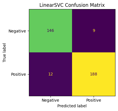
# Confusion matrix
fig, ax = plt.subplots(figsize=(5, 4))
ConfusionMatrixDisplay.from_predictions(y_te, y_pred_linear,
    display_labels=['Negative', 'Positive'], colorbar=False, ax=ax)
ax.set_title('LinearSVC Confusion Matrix')
plt.tight_layout()
plt.show()

# Top positive and negative weights
coef = linear_svc.coef_[0]
feature_names = np.array(tfidf.get_feature_names_out())
print("\nTop 10 words predicting POSITIVE class:")
print(', '.join(feature_names[np.argsort(coef)[-10:]][::-1]))
print("\nTop 10 words predicting NEGATIVE class:")
print(', '.join(feature_names[np.argsort(coef)[:10]]))

=== LinearSVC ===
              precision    recall  f1-score   support

    Negative       0.92      0.94      0.93       155
    Positive       0.95      0.94      0.95       200

    accuracy                           0.94       355
   macro avg       0.94      0.94      0.94       355
weighted avg       0.94      0.94      0.94       355


Top 10 words predicting POSITIVE class:
hockey, game, team, games, roger, teams, nhl, player, players, mask

Top 10 words predicting NEGATIVE class:
clinton, people, of, government, law, we, that, and, part, your

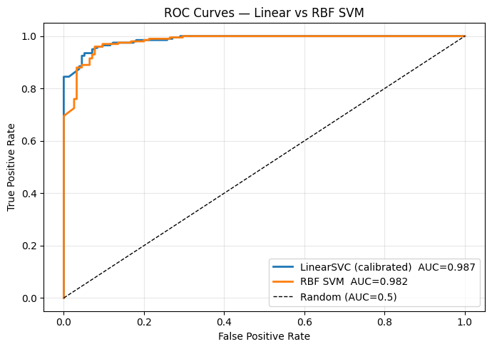
4. RBF Kernel SVM and ROC Comparison¶

Linear SVMs work well for text, but let’s compare with RBF to see if non-linear patterns exist.

%matplotlib inline
from sklearn.svm import SVC
from sklearn.metrics import roc_curve, auc
import matplotlib.pyplot as plt
import numpy as np

# RBF SVM (on reduced features for speed)
from sklearn.decomposition import TruncatedSVD
svd = TruncatedSVD(n_components=200, random_state=42)
X_tr_reduced = svd.fit_transform(X_tr)
X_te_reduced = svd.transform(X_te)

rbf_svc = SVC(kernel='rbf', C=10.0, gamma='scale', probability=True, random_state=42)
rbf_svc.fit(X_tr_reduced, y_tr)
y_pred_rbf = rbf_svc.predict(X_te_reduced)
y_prob_rbf = rbf_svc.predict_proba(X_te_reduced)[:, 1]

# LinearSVC probabilities via decision function (Platt scaling)
from sklearn.calibration import CalibratedClassifierCV
calib_linear = CalibratedClassifierCV(LinearSVC(C=1.0, max_iter=5000, random_state=42), cv=3)
calib_linear.fit(X_tr, y_tr)
y_prob_linear = calib_linear.predict_proba(X_te)[:, 1]

# ROC curves
fig, ax = plt.subplots(figsize=(7, 5))
for name, y_prob in [('LinearSVC (calibrated)', y_prob_linear), ('RBF SVM', y_prob_rbf)]:
    fpr, tpr, _ = roc_curve(y_te, y_prob)
    roc_auc = auc(fpr, tpr)
    ax.plot(fpr, tpr, lw=2, label=f'{name}  AUC={roc_auc:.3f}')
ax.plot([0,1],[0,1],'k--',lw=1,label='Random (AUC=0.5)')
ax.set_xlabel('False Positive Rate'); ax.set_ylabel('True Positive Rate')
ax.set_title('ROC Curves — Linear vs RBF SVM')
ax.legend(); ax.grid(alpha=0.3)
plt.tight_layout()
plt.show()

from sklearn.metrics import classification_report
print("=== RBF SVM (SVD features) ===")
print(classification_report(y_te, y_pred_rbf, target_names=['Negative', 'Positive']))

=== RBF SVM (SVD features) ===
              precision    recall  f1-score   support

    Negative       0.95      0.90      0.93       155
    Positive       0.93      0.96      0.95       200

    accuracy                           0.94       355
   macro avg       0.94      0.93      0.94       355
weighted avg       0.94      0.94      0.94       355

5. Error Analysis — What Does the Model Get Wrong?¶

%matplotlib inline
import numpy as np
import matplotlib.pyplot as plt

# Re-run calibrated linear for probabilities
y_pred_cal = calib_linear.predict(X_te)
y_prob_cal = calib_linear.predict_proba(X_te)[:, 1]

# False positives and false negatives
fp_idx = np.where((y_pred_cal == 1) & (y_te == 0))[0]
fn_idx = np.where((y_pred_cal == 0) & (y_te == 1))[0]

print(f"False positives: {len(fp_idx)}  (predicted Positive, actually Negative)")
print(f"False negatives: {len(fn_idx)}  (predicted Negative, actually Positive)")

print("\nSample FALSE POSITIVES (confident wrong predictions):")
fp_sorted = fp_idx[np.argsort(y_prob_cal[fp_idx])[-3:][::-1]]
for i in fp_sorted:
    print(f"  [prob={y_prob_cal[i]:.3f}] {X_te_raw[i][:200].strip()}")
    print()

print("\nSample FALSE NEGATIVES (confident wrong predictions):")
fn_sorted = fn_idx[np.argsort(y_prob_cal[fn_idx])[:3]]
for i in fn_sorted:
    print(f"  [prob={y_prob_cal[i]:.3f}] {X_te_raw[i][:200].strip()}")
    print()

False positives: 11  (predicted Positive, actually Negative)
False negatives: 11  (predicted Negative, actually Positive)

Sample FALSE POSITIVES (confident wrong predictions):
  [prob=0.703] I notice you did not offer an alternative number.  Try this one on for
size..... by the year 2000, American taxpayers will have given Israel
one dollar for every star in the Milky Way Galaxy.

  [prob=0.680] When did Bill start doing endorsements?

         Will he do the "Remington Shaver" ad?

  [prob=0.677] 


Sample FALSE NEGATIVES (confident wrong predictions):
  [prob=0.057] Do you realize how many smiles are crossing faces after you wrote that?
(-;

gld

  [prob=0.068] Here is a press release from the White House.

 Remarks by President Clinton to NCAA Division I Champion Hockey Team
April 19; Q&A Following
 To: National Desk
 Contact: White House Office of the Pres

  [prob=0.072] Well, so are we, and we see it completely different than you. Guess it's a
matter of perspective.

6. Try It in the Browser¶

Classify a short text review using a simple bag-of-words + linear rule.

def tokenise(text):
    import re
    return re.findall(r'[a-z]+', text.lower())

# Learned positive/negative indicator words (simplified)
positive_words = {'great', 'excellent', 'love', 'amazing', 'fantastic', 'best', 'perfect', 'good', 'wonderful', 'happy'}
negative_words = {'terrible', 'awful', 'hate', 'horrible', 'worst', 'bad', 'poor', 'boring', 'useless', 'slow'}

def predict_sentiment(review):
    tokens = set(tokenise(review))
    pos_hits = tokens & positive_words
    neg_hits = tokens & negative_words
    score = len(pos_hits) - len(neg_hits)
    label = 'POSITIVE' if score >= 0 else 'NEGATIVE'
    return label, score, list(pos_hits), list(neg_hits)

reviews = [
    "This product is fantastic and works perfectly, great value!",
    "Absolutely terrible quality, worst purchase I have ever made.",
    "It arrived on time but the battery life is poor and the design is boring.",
]
for r in reviews:
    label, score, pos, neg in [predict_sentiment(r)]:
        print(f"Review : {r[:60]}...")
        print(f"Label  : {label}  (score={score})")
        print(f"Pos words: {pos}  |  Neg words: {neg}")
        print()

Knowledge Check¶

Why is `LinearSVC` preferred over `SVC(kernel='linear')` for large text datasets?¶

[ ] A) It uses a different loss function [ ] B) It solves the primal directly with liblinear, scaling O(n·p) instead of O(n²) for the kernel dual [ ] C) It always produces higher accuracy [ ] D) It supports probability estimates natively

Check

The TF-IDF sublinear_tf=True parameter applies $\log(1 + f_{t,d})$ instead of raw frequency. This helps because:¶

[ ] A) It increases the dimensionality of the feature space [ ] B) It reduces the disproportionate weight of very frequent terms like "the" [ ] C) It makes the Gram matrix PSD [ ] D) It normalises the labels to [-1, 1]

Check

Exercises¶

Exercise 1 — Pipeline with C Tuning¶

Build a Pipeline([('tfidf', TfidfVectorizer(...)), ('svm', LinearSVC(...))]) and use GridSearchCV over C ∈ [0.01, 0.1, 1, 10]. Report the best C and its cross-validated F1.

Exercise 2 — Threshold Optimisation¶

Using the calibrated linear SVM probabilities (predict_proba), sweep thresholds from 0.1 to 0.9. Plot precision vs recall vs threshold. At what threshold does F1 peak for the positive class?

Exercise 3 — Feature Importance Bar Chart¶

Plot the top 15 words by LinearSVC coefficient magnitude (absolute value), coloured by sign (positive/negative class). What business insight do the top words reveal?

%matplotlib inline
# Exercise 1, 2, 3: your code here
from sklearn.svm import LinearSVC
from sklearn.feature_extraction.text import TfidfVectorizer
from sklearn.pipeline import Pipeline
from sklearn.model_selection import GridSearchCV
# Your code here

Common Pitfalls¶

What’s Next¶

Congratulations — you have completed the Support Vector Machines chapter. You have built:

Maximum-margin linear classifiers
Kernel SVMs (RBF, polynomial, custom)
Soft-margin regularisation with the C parameter
An end-to-end NLP sentiment classifier

The next chapter covers ensemble methods — Random Forests and Gradient Boosting — where multiple weak learners combine to outperform any single model. These techniques dominate structured/tabular ML competitions and are the backbone of most production ML systems.