Calculus Essentials - Machine Learning for Business

Welcome to Calculus Essentials, the notebook where machine learning stops being a static formula and starts becoming a learning system.

Linear algebra gave us the language for data tables and weighted combinations. Calculus adds motion: it tells us how prediction error changes when we nudge a parameter, which direction improves the model, and how fast we should move.

Why This Matters in Business ML¶

Calculus shows up whenever a business model needs to improve itself:

Calculus idea	ML role	Business question it answers
Derivative	Measures local change	If price changes slightly, how does profit respond?
Gradient	Direction of steepest change	Which lever should we adjust first?
Minimum / maximum	Best operating point	Where is cost lowest or profit highest?
Integral	Accumulated change	What total effect builds up over time?

We will mainly use one simple cost function throughout the notebook so the ideas stay connected rather than scattered.

Visual Intuition: How Models Learn¶

A training loop is really a repeated calculus story: predict, measure error, inspect the slope, then update parameters.

Alt text: A loop shows parameters being updated after loss and gradient are computed.

In business language: calculus gives the model a disciplined way to learn from mistakes instead of changing settings randomly.

Worked Example: A Simple Cost Function¶

To keep the notebook coherent, we will reuse a single business example:

C(q) = 5q^2 - 40q + 200

(1)

where $q$ is the production quantity and $C(q)$ is total cost.

This one function is enough to illustrate:

limits
continuity
differentiation
minima
gradient descent

At $q = 4$ :

C(4) = 5(4)^2 - 40(4) + 200 = 120

(2)

We will return to this value several times because it turns out to be the lowest point of the curve.

Limits and Continuity¶

A limit asks what value a function approaches as the input gets close to a point.

For our cost function:

\lim_{q \to 4} C(q) = \lim_{q \to 4}(5q^2 - 40q + 200) = 120

(3)

Because this is a polynomial, it is continuous for every real value of $q$ . That means there are no jumps, holes, or breaks in the curve.

\lim_{q \to a} C(q) = C(a)

(4)

This matters in ML because gradient-based training assumes small parameter changes lead to small, understandable changes in the loss surface.

A quick example at $q=5$ gives:

C(5) = 5(5)^2 - 40(5) + 200 = 125

(5)

Differentiation and Marginal Change¶

The derivative measures how fast a function changes at a specific point.

For the cost function, the first derivative is:

C'(q) = \frac{d}{dq} C(q) = 10q - 40

(6)

This derivative is the marginal cost: the approximate change in total cost when production increases by one more unit.

At $q = 6$ :

C'(6) = 10(6) - 40 = 20

(7)

So near $q=6$ , adding one more unit increases cost by about 20 currency units.

Interpreting the Sign of the Derivative¶

If $C'(q) > 0$ , cost is increasing at that point.
If $C'(q) < 0$ , cost is decreasing at that point.
If $C'(q) = 0$ , the curve is locally flat, so we may be at a minimum or maximum.

This is the key bridge to ML: the derivative acts like a local compass.

Minima, Maxima, and the Best Operating Point¶

To find the quantity that minimizes cost, set the derivative to zero:

C'(q) = 0 \Rightarrow 10q - 40 = 0 \Rightarrow q = 4

(8)

Then check the second derivative:

C''(q) = 10 > 0

(9)

A positive second derivative means the curve bends upward, so $q=4$ is a minimum.

Therefore, the minimum total cost is:

C(4) = 120

(10)

This same logic appears in ML when we search for parameters that minimize loss rather than production cost.

Business reading	ML reading
Find the cheapest production point	Find the lowest-loss parameter setting
Marginal cost becomes zero	Gradient becomes zero
Curvature confirms a minimum	Curvature helps diagnose the landscape

Gradient Descent¶

In machine learning, we usually do not solve every optimization problem analytically. Instead, we use an iterative rule that repeatedly moves in the direction that reduces loss.

For our cost function, gradient descent updates quantity using:

q_{new} = q_{old} - \eta \cdot C'(q_{old})

(11)

where $\eta$ is the learning rate.

If we start from $q=8$ and use $\eta = 0.1$ , the update keeps moving us toward $q=4$ because the derivative points uphill and gradient descent always steps the other way.

Two practical lessons carry directly into ML:

a learning rate that is too large can overshoot the minimum
a learning rate that is too small may converge safely but very slowly

Additional Intuition: Physics and Accumulation¶

A second way to interpret calculus is through motion.

If position is

s(t) = t^2 + 2t + 1

(12)

then velocity is the derivative of position and acceleration is the derivative of velocity:

v(t) = s'(t) = 2t + 2, \qquad a(t) = v'(t) = 2

(13)

This lens is useful because it makes the derivative feel less abstract: it is a rate of change, whether that rate describes moving objects, changing costs, or changing loss values in training.

Integration as Accumulated Effect¶

Integration reverses differentiation. If derivatives tell us the local rate, integrals accumulate those local pieces back into a total effect.

For example:

\int (x + 1) \, dx = \frac{x^2}{2} + x + C

(14)

In business terms, you can think of integration as summing many small changes to recover a total quantity such as total cost, total revenue, or cumulative profit.

We will not go deep into advanced integration here; the goal is to recognize its role and defer heavier worked examples to the math cheat-sheet notebook.

Where the Power Rule Comes From¶

The power rule is one of the most useful shortcuts in introductory calculus:

\frac{d}{dx}(x^n) = nx^{n-1}

(15)

It comes from the derivative definition:

\frac{d}{dx}f(x) = \lim_{h \to 0} \frac{f(x+h) - f(x)}{h}

(16)

If $f(x)=x^n$ , expanding $(x+h)^n$ with the binomial theorem leaves one surviving term after dividing by $h$ and taking the limit, which produces $nx^{n-1}$ .

The reverse rule for antiderivatives is:

\int x^n \, dx = \frac{x^{n+1}}{n+1} + C \qquad (n \neq -1)

(17)

You do not need to memorize the derivation in full for ML, but you do need the interpretation: derivatives tell you how things change locally, while integrals help accumulate those changes back into totals.

Guided Practice and Exercises¶

Quick Check¶

What does the derivative tell us at a point?

(A) The exact future value of the function
(B) The local slope or rate of change
(C) The area under the whole curve

If the learning rate is too large in gradient descent, what usually happens?

(A) The algorithm may overshoot the minimum
(B) The derivative becomes zero immediately
(C) The function stops being continuous

Why is continuity helpful for optimization?

(A) It guarantees every function is linear
(B) It avoids abrupt jumps that break local slope reasoning
(C) It removes the need for a loss function

Exercises¶

Compute $C'(q)$ and evaluate it at $q=2$ , $q=4$ , and $q=7$ . Explain what each sign means in plain language.
Change the learning rate in the gradient descent code from 0.1 to 0.01 and then to 0.4. Compare the speed and stability of convergence.
Rewrite the optimization example for a profit function instead of a cost function. What changes when you want to maximize rather than minimize?

Key Takeaways¶

derivatives measure local change
minima are found where slope becomes zero and curvature confirms the valley
gradient descent converts calculus into a repeatable learning rule
these same ideas power optimization across modern ML

Bridge to the Next Notebook¶

Calculus explains how models move across an error surface. The next notebook shifts from change to uncertainty.

In other words: calculus helps a model learn; probability helps it reason under imperfect information.

Next stop: Probability Essentials

import numpy as np
import matplotlib.pyplot as plt

def cost(q):
    return 5 * q**2 - 40 * q + 200

def numerical_derivative(func, x, h=1e-3):
    return (func(x + h) - func(x)) / h

def visualize_derivative_and_area(func, x_point=4.0, a=0.0, b=6.0, n_rectangles=20):
    x_vals = np.linspace(a - 1, b + 1, 400)
    y_vals = func(x_vals)

    slope = numerical_derivative(func, x_point)
    y_point = func(x_point)
    tangent = slope * (x_vals - x_point) + y_point

    x_rect = np.linspace(a, b, n_rectangles + 1)
    dx = (b - a) / n_rectangles
    midpoints = (x_rect[:-1] + x_rect[1:]) / 2
    heights = func(midpoints)
    approx_area = np.sum(heights * dx)

    fig, axes = plt.subplots(1, 2, figsize=(12, 4))

    axes[0].plot(x_vals, y_vals, label='C(q)')
    axes[0].plot(x_vals, tangent, '--', label=f'Tangent at q={x_point}')
    axes[0].scatter([x_point], [y_point], color='crimson', zorder=5)
    axes[0].set_title('Derivative as a local slope')
    axes[0].set_xlabel('q')
    axes[0].set_ylabel('Cost')
    axes[0].legend()
    axes[0].grid(True, alpha=0.3)

    axes[1].plot(x_vals, y_vals, label='C(q)')
    axes[1].bar(x_rect[:-1], heights, width=dx, alpha=0.5, align='edge', edgecolor='black', label=f'Approx. area = {approx_area:.1f}')
    axes[1].set_title('Integral as accumulated area')
    axes[1].set_xlabel('q')
    axes[1].set_ylabel('Cost')
    axes[1].legend()
    axes[1].grid(True, alpha=0.3)

    plt.tight_layout()
    plt.show()

visualize_derivative_and_area(cost, x_point=4.0, a=0.0, b=6.0, n_rectangles=16)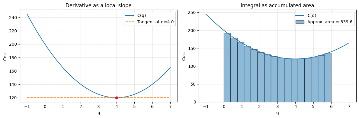

import numpy as np
import matplotlib.pyplot as plt

def cost(q):
    return 5 * q**2 - 40 * q + 200

def grad_cost(q):
    return 10 * q - 40

def gradient_descent(start_q=8.0, eta=0.1, steps=20):
    qs = [start_q]
    costs = [cost(start_q)]
    q = start_q
    for _ in range(steps):
        q = q - eta * grad_cost(q)
        qs.append(q)
        costs.append(cost(q))
    return np.array(qs), np.array(costs)

qs, costs = gradient_descent(start_q=8.0, eta=0.1, steps=20)
q_space = np.linspace(-1, 10, 400)

fig, axes = plt.subplots(1, 2, figsize=(12, 4))
axes[0].plot(q_space, cost(q_space), label='C(q)')
axes[0].scatter(qs, costs, c=np.arange(len(qs)), cmap='viridis', zorder=5)
axes[0].set_title('Gradient descent path')
axes[0].set_xlabel('q')
axes[0].set_ylabel('Cost')
axes[0].legend()
axes[0].grid(True, alpha=0.3)

axes[1].plot(range(len(costs)), costs, '-o')
axes[1].set_title('Cost by iteration')
axes[1].set_xlabel('Iteration')
axes[1].set_ylabel('Cost')
axes[1].grid(True, alpha=0.3)

plt.tight_layout()
plt.show()

print(f'Final q: {qs[-1]:.4f}')
print(f'Final cost: {costs[-1]:.4f}')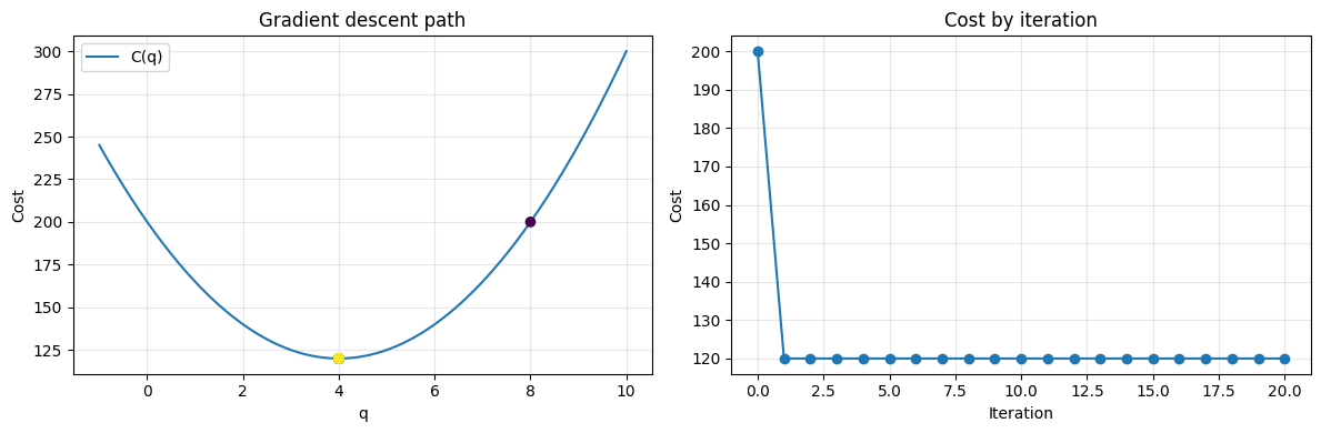

Final q: 4.0000
Final cost: 120.0000